3 de la Croix and Dottori (2008)

This section discusses Croix and Dottori (2008), using a simplified model to illustrate the key points.

3.1 Introduction

This paper analyses the very different population patterns of two remote islands in the Pacific Ocean: Easter Island and Tikopia. While Tikopians managed to control population growth and natural-resource use, the inhabitants of Easter Island engaged in clan competition for control of resources, leading to overpopulation and overexploitation of resources.

A key aspect of this paper is the special role of fertility. Most papers assume that parents derive some utility from having children. However, in de la Croix and Dottori, fertility is chosen strategically before a Nash bargaining process over the control of resources. In particular, a larger population, facilitated by having more children, raises the value of the fallback option during the negotiation process. Consequently, individuals optimally decide to have more children, because this implies a better bargaining position. In this sense, equilibrium fertility rates result from the complementarities between different groups’ fertility decisions. In the paper’s general model, the fertility externality can generate a population race, exhaust natural resources and produce an environmental collapse. The special case studied below is deliberately simpler: its clan populations converge to a finite common level, so it illustrates strategic convergence rather than population explosion.

3.1.1 Historical data

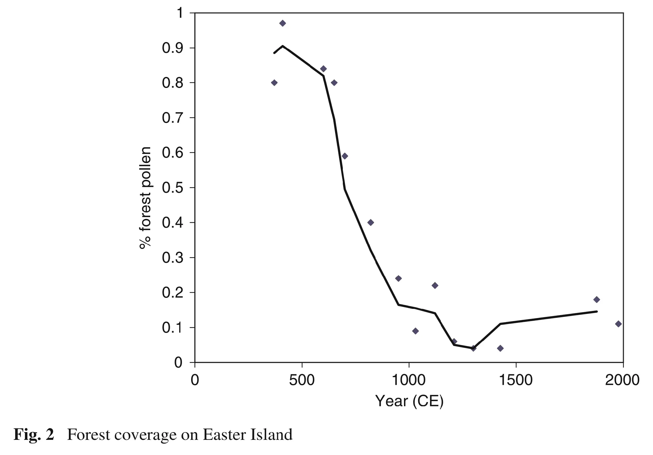
Based on the archaeological estimates reported in the paper, Easter Island’s population increased very little between 400 CE (about 100 people) and 1100 CE. It then grew rapidly, reaching about 10,000 people during 1400–1600 CE. The effects of the population race were apparent by 1600 CE: food consumption declined and the population fell sharply during the seventeenth century. By 1722, when Europeans arrived at Easter Island, the total population was around 3,000 people. In parallel, evidence about Easter Island’s forests indicates that tree cutting began after the first settlers arrived around 400 CE. By 1400 CE, deforestation had reached its peak, and when Europeans arrived there were almost no trees on the island.

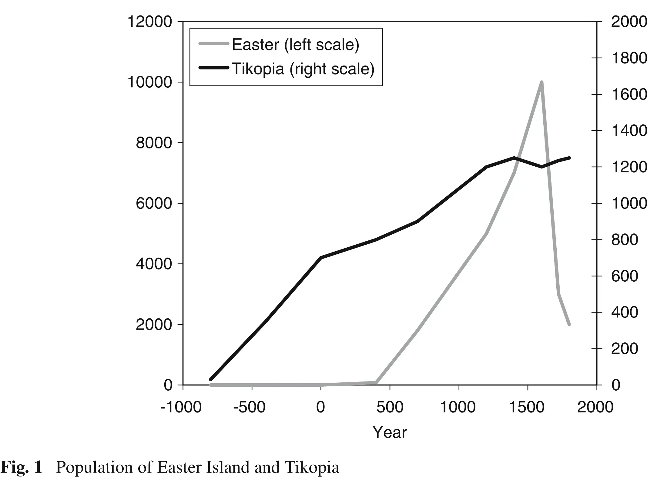
Figure 1 in de la Croix and Dottori, 2008

Figure 2 in de la Croix and Dottori, 2008

Meanwhile, Tikopia was settled around 900 BCE, and its inhabitants practised slash-and-burn agriculture. By 100 BCE, diminishing returns from natural resources led to pig breeding. This lasted until the seventeenth century, when Tikopians abandoned it because pigs required too many resources. The total population stabilised at around 1,200 people and was kept at that level through deliberate mechanisms, including celibacy, abortion, infanticide and sea voyages by young men.

3.2 The model

De la Croix and Dottori use an OLG framework. In the paper, agents live for two periods. However, important decisions are taken at the clan level, which acts as a representative agent. Clans (and individuals) are rational, have perfect foresight and take the actions of the other clan as given. The timing is as follows:

Each clan chooses its fertility level.
A Nash-Cournot fertility equilibrium arises.
Crops are cultivated and shared between clans following a non-cooperative bargaining process.

For simplicity, the island is populated by two opposing clans; every individual belongs to exactly one clan and cannot change clans.

The paper’s general model contains four parameters that matter for the population race. Conflict success depends on relative clan size according to \[ \pi_t=\frac{N_{1,t}^{\mu}}{N_{1,t}^{\mu}+N_{2,t}^{\mu}}, \] where \(\mu>0\) measures how responsive Group 1’s probability of victory is to relative numbers. Aggregate production is \[ Y_t=A(R_t)L^{\alpha}(N_{1,t}+N_{2,t})^{1-\alpha}, \] where \(L\) is fixed land and \(\alpha\in(0,1]\) is the land share. War destroys a fraction \(\omega\in[0,1]\) of the crop, so the disagreement shares of the original crop are \((1-\omega)\pi_t\) for Group 1 and \((1-\omega)(1-\pi_t)\) for Group 2. Raising children also has a current cost \(\lambda n_{i,t}\), with \(\lambda\geq0\); in the general budget, young consumption is \[ c_{i,t}=\left(1-\frac{\tau}{1+n_{i,t-1}}-\lambda n_{i,t}\right)y_{i,t}. \] The Nash bargaining solution therefore assigns Group 1 the crop share \[ \theta_t=\gamma\omega+(1-\omega)\pi_t, \] where \(\gamma\in(0,1)\) is Group 1’s Nash bargaining weight.

To obtain transparent closed-form dynamics, the remainder of this section imposes the following special case before using population shares, linear production and the cube-root fertility rules: \[ \tag{Assumption 1} \mu=1,\qquad \omega=0,\qquad \lambda=0,\qquad \alpha=1. \] Thus \(\pi_t\) is Group 1’s population share, \(Y_t=A(R_t)L\), and \(\theta_t=\pi_t\). These restrictions are stronger than the assumptions behind the paper’s general environmental-collapse result.

3.2.1 Preferences

Clan \(i\) at time \(t\) consists of \(N_{i,t}\) adults. Adults work, support their parents and have children. Old agents only consume what their children provide for them.¹ Total utility is given by: \[ U_{i,t} = c_{i,t} + \beta d_{i,t+1}, \]

where \(c_{i,t}\) and \(d_{i,t+1}\) represent consumption when young and old, respectively.

3.2.2 Budget

The income of an adult agent is \(y_{i,t}\). Each adult supports their parents by giving them some resources. Support for parents depends on the number of siblings. In particular, each sibling contributes the following share of their income: \[ \frac{\tau}{1+n_{i,t-1}}, \]

where \(\tau \in (0,1)\). Clearly, the contribution decreases with the number of siblings.

Consequently, an agent who had \(n_{i,t}\) children receives the following total support in old age:

\[ d_{i,t+1} = n_{i,t}\frac{\tau}{1+n_{i,t}}y_{i,t+1}. \]

Under Assumption 1, \(\lambda=0\). Since income is divided between consumption and support for parents, \(y_{i,t}=c_{i,t}+\frac{\tau}{1+n_{i,t-1}}y_{i,t}\), consumption when young is therefore

\[ c_{i,t} = \left( 1 - \frac{\tau}{1+n_{i,t-1}}\right)y_{i,t}. \]

3.2.3 Population

The population of each clan evolves according to the chosen fertility level: \[ N_{i,t+1} = N_{i,t}n_{i,t}. \]

3.2.4 Production

Under Assumption 1, labour has a zero exponent, land is fixed at \(L\), and total factor productivity depends on the available natural resources \(R_t\). The general production function above consequently reduces to \[ Y_t=A(R_t)L. \]

The dynamics of resources follow the paper by Matsumoto (2002): \[ R_{t+1} = \left(1 +\delta - \delta \frac{R_t}{K} - b (N_{1,t} + N_{2,t})\right)R_t, \]

where \(K>0\) is the carrying capacity, \(\delta>0\) is the intrinsic growth rate of resources and \(b>0\) measures population pressure on resources.

3.3 Bargaining

Bargaining uses the Nash solution. For \(\omega>0\), it maximises

\[ (U_{1,t}- \bar{U}_{1,t})^\gamma(U_{2,t} - \bar{U}_{2,t})^{1-\gamma}, \]

where \(U_{i,t}\) is Group \(i\)’s utility under agreement and \(\bar U_{i,t}\) is its disagreement utility. Under Assumption 1, the probability that Group 1 wins is its population share:

\[ \pi_t = \frac{N_{1,t}}{N_{1,t} + N_{2,t}}. \]

Thus a larger clan is more likely to win a war. Increasing population also improves the clan’s bargaining position by raising its disagreement utility.

To derive the general sharing rule, temporarily retain \(\omega\) and \(\lambda\). Suppose the clans agree on a crop share \(\theta_t\): Group 1 receives \(\theta_t\), and Group 2 receives the remaining \(1-\theta_t\). Indirect utilities are then

\[ U_{1,t} = \left(1-\frac{\tau}{1+n_{1,t-1}}-\lambda n_{1,t}\right)\frac{\theta_tY_t}{N_{1,t}}+\beta\frac{n_{1,t}\tau}{1+n_{1,t}}\frac{\theta_{t+1}Y_{t+1}}{N_{1,t+1}}, \] \[ U_{2,t} = \left(1-\frac{\tau}{1+n_{2,t-1}}-\lambda n_{2,t}\right)\frac{(1-\theta_t)Y_t}{N_{2,t}}+\beta\frac{n_{2,t}\tau}{1+n_{2,t}}\frac{(1-\theta_{t+1})Y_{t+1}}{N_{2,t+1}}. \]

In the general model, war destroys the fraction \(\omega\) of current production. The disagreement shares are therefore \((1-\omega)\pi_t\) and \((1-\omega)(1-\pi_t)\). The current-period parts of the disagreement utilities are

\[ \bar{U}_{1,t} = (1-\omega)\pi_t\left(1-\frac{\tau}{1+n_{1,t-1}}-\lambda n_{1,t}\right)\frac{Y_t}{N_{1,t}}+\beta\frac{n_{1,t}\tau}{1+n_{1,t}}\frac{\theta_{t+1}Y_{t+1}}{N_{1,t+1}}, \] \[ \bar{U}_{2,t} = (1-\omega)(1-\pi_t)\left(1-\frac{\tau}{1+n_{2,t-1}}-\lambda n_{2,t}\right)\frac{Y_t}{N_{2,t}}+\beta\frac{n_{2,t}\tau}{1+n_{2,t}}\frac{(1-\theta_{t+1})Y_{t+1}}{N_{2,t+1}}. \]

The agreement surpluses that depend on \(\theta_t\) are proportional to

\[ U_{1,t}-\bar{U}_{1,t}=\left(1-\frac{\tau}{1+n_{1,t-1}}-\lambda n_{1,t}\right)\left[\theta_t-(1-\omega)\pi_t\right]\frac{Y_t}{N_{1,t}}, \] \[ U_{2,t}-\bar{U}_{2,t}=\left(1-\frac{\tau}{1+n_{2,t-1}}-\lambda n_{2,t}\right)\left[1-\theta_t-(1-\omega)(1-\pi_t)\right]\frac{Y_t}{N_{2,t}}. \]

At the time of bargaining, the positive factors \(\left(1-\frac{\tau}{1+n_{i,t-1}}-\lambda n_{i,t}\right)Y_t/N_{i,t}\) are predetermined. Maximising over \(\theta_t\) therefore gives \[ \theta_t=\gamma\omega+(1-\omega)\pi_t. \]

Assumption 1 sets \(\omega=0\). In that case no crop is lost in war, the feasible individually rational set collapses to the single allocation \(\theta_t=\pi_t\), and both agreement surpluses are zero. Thus the usual positive-surplus Nash product is degenerate; \(\theta_t=\pi_t=N_{1,t}/(N_{1,t}+N_{2,t})\) should be understood as the limit of the general solution as \(\omega\downarrow0\), not as the maximiser of an invalid zero-surplus Nash product.

3.4 Fertility

We can now compute fertility in the Assumption 1 special case. At time \(t\), current population and the current sharing rule are predetermined. Group 1 therefore solves

\[ \begin{aligned} \max_{n_{1,t}}\quad &\underbrace{\left(1-\frac{\tau}{1+n_{1,t-1}}\right)\frac{\theta_tY_t}{N_{1,t}}}_{\text{constant at }t} \\ &+\frac{\beta\tau n_{1,t}}{1+n_{1,t}} \left[\frac{N_{1,t}n_{1,t}}{N_{1,t}n_{1,t}+N_{2,t}n_{2,t}}\right] \frac{A(R_{t+1})L}{N_{1,t}n_{1,t}}. \end{aligned} \]

Group 2’s current share is \(1-\theta_t\), and its future share and future population are based on Group 2, not Group 1. Its corresponding problem is \[ \begin{aligned} \max_{n_{2,t}}\quad &\underbrace{\left(1-\frac{\tau}{1+n_{2,t-1}}\right)\frac{(1-\theta_t)Y_t}{N_{2,t}}}_{\text{constant at }t} \\ &+\frac{\beta\tau n_{2,t}}{1+n_{2,t}} \left[\frac{N_{2,t}n_{2,t}}{N_{1,t}n_{1,t}+N_{2,t}n_{2,t}}\right] \frac{A(R_{t+1})L}{N_{2,t}n_{2,t}}. \end{aligned} \]

After cancelling future own-group population from each crop share and per-capita income, the fertility-dependent terms are proportional to \[ \frac{n_{i,t}}{(1+n_{i,t})(N_{1,t}n_{1,t}+N_{2,t}n_{2,t})}. \] The first-order conditions give the best responses \[ n_{1,t}^{2}=\frac{N_{2,t}}{N_{1,t}}n_{2,t}, \qquad n_{2,t}^{2}=\frac{N_{1,t}}{N_{2,t}}n_{1,t}. \] Solving these two conditions simultaneously gives the equilibrium fertility levels

\[ n^\star_{1,t} = \left(\frac{N_{2,t}}{N_{1,t}}\right)^\frac{1}{3}, \] \[ n^\star_{2,t} = \left(\frac{N_{1,t}}{N_{2,t}}\right)^\frac{1}{3}, \]

Thus Group 1’s equilibrium fertility is higher when Group 2 is relatively more populous, and conversely. This strategic response is the population-race mechanism. In the paper’s general model it can amplify total population and environmental pressure. Under Assumption 1, however, the population dynamics below equalise two finite clan populations; they do not generate population explosion. Population still affects the resource stock through \[ R_{t+1} = \left(1 +\delta - \delta \frac{R_t}{K} - b (N_{1,t} + N_{2,t})\right)R_t, \]

3.5 Steady-state population and natural resources

For the Assumption 1 special case, we can compute the steady-state population using the two dynamic equations:

\[ n^\star_{1,t} = \left(\frac{N_{2,t}}{N_{1,t}}\right)^\frac{1}{3} \implies N_{1,t+1} = N_{1,t}\left(\frac{N_{2,t}}{N_{1,t}}\right)^\frac{1}{3} \] \[ n^\star_{2,t} = \left(\frac{N_{1,t}}{N_{2,t}}\right)^\frac{1}{3} \implies N_{2,t+1} = N_{2,t}\left(\frac{N_{1,t}}{N_{2,t}}\right)^\frac{1}{3}, \]

It is simpler to solve the corresponding linearised system, which we can obtain by taking logarithms: \[ \tilde{N}_{i,t+1} = \frac{2}{3}\tilde{N}_{i,t} + \frac{1}{3} \tilde{N}_{j,t}, \] where \(\tilde{N}_{i,t}=\log N_{i,t}\).

We can obtain the dynamics of the logarithmic system:

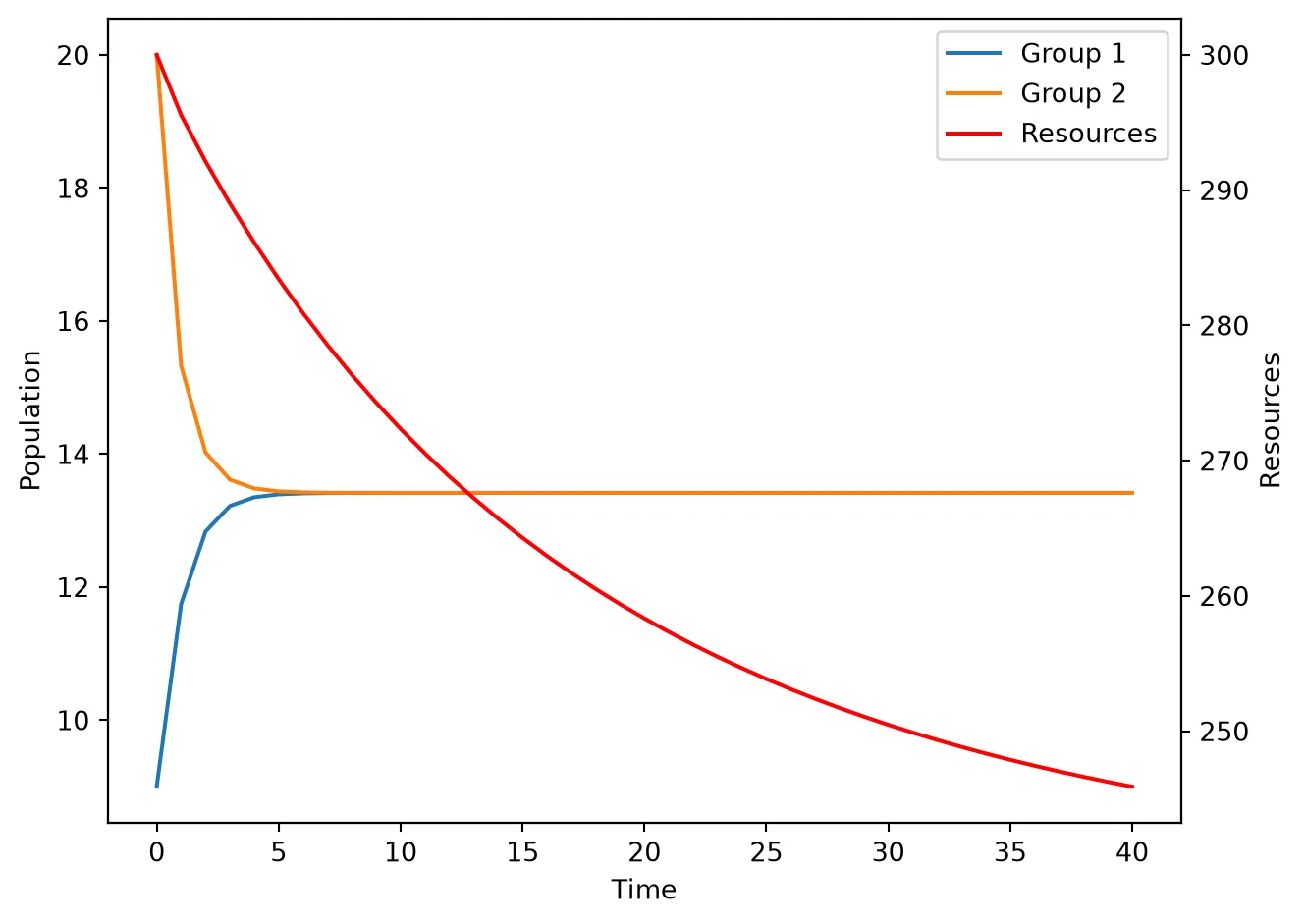
\[ \tilde{N}_{i,t} = \frac{\tilde{N}_{i,0} + \tilde{N}_{j,0}}{2} + \frac{1}{2} 3^{-t}\left( \tilde{N}_{i,0} - \tilde{N}_{j,0} \right). \] The population of each clan converges to the finite common level \[ \bar{N}_i = \bar{N}_j = \sqrt{N_{1,0}}\sqrt{N_{2,0}}, \]

If \(b(\bar N_i+\bar N_j)<\delta\), the corresponding positive steady-state level of natural resources is

\[ \bar{R} = K\left(1-\frac{b(\bar{N}_i+\bar{N}_j)}{\delta}\right). \]

3.5.1 Simulated trajectory

Lastly, we can compute the trajectory of the special-case system for a set of parameters to visualise the evolution of the main variables. For instance, take \(N_{1,0}=9\), \(N_{2,0}=20\), \(\delta=0.08\), \(K=400\), \(b=0.0012\) and \(R_0=300\).

Figure 3.1: Simulated trajectory of populations and resources over time

In a sense, in this model individuals save by having children.↩︎