4 Galor and Moav (2006)
This section discusses the work of Galor and Moav (2006), which presents an OLG model to explain the rise of publicly financed education and the transition from a class structure characterised by capitalists and workers to an economy in which both groups own capital.
The paper proposes that the demise of this class division was a deliberate action on the part of capitalists to sustain their profits as human capital became increasingly important in production. That is, at some point human capital becomes really necessary for production, and capitalists find it optimal to tax themselves to finance workers’ education. Doing so raises the level of human capital and allows them to sustain their profits.
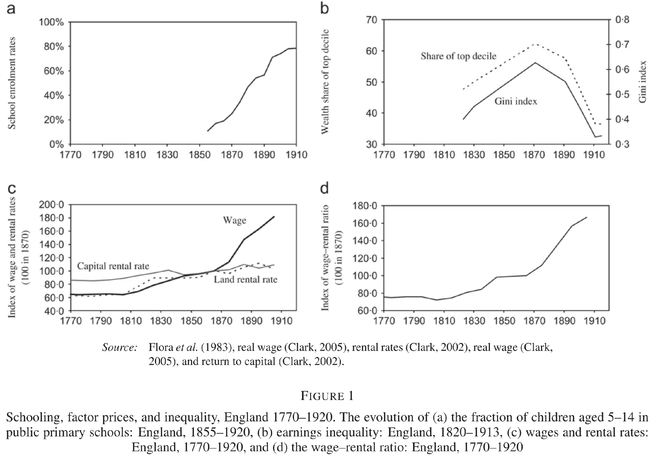
The mechanism is intended to describe the later stages of industrialisation and the transition to the beginning of the twentieth century. Figure 1 covers England from 1770 to 1920. It shows that inequality first rose during the early stages of industrialisation and then fell, while school enrolment increased strongly during the later decline in inequality. The theory the authors propose parallels this evolution. Furthermore, they supplement the model with econometrics that are compatible with the predictions of the model.
4.1 The model
We present a simplified version of the model using precise functional forms for the human capital accumulation process and the production function. Our presentation comprises two sections: * The general model * The application of the model to a society with two classes. We will follow this approach.
For the moment, the economy comprises only one type of individual. Individuals live for two periods of time: young and adult. Young individuals do not produce and use their time to acquire human capital. If education is provided, human capital accumulation is faster.
4.1.1 Production and prices
A single homogeneous good is produced using physical and human capital according to a Cobb-Douglas production function. In particular:
\[ Y_t = F(H_t, K_t) = A K_t^\alpha H_t^{1-\alpha} = H_t A k_t^\alpha,\quad k_t \equiv \frac{K_t}{H_t}. \]
Thus, aggregate output is \(Y_t=H_t f(k_t)\), where output per efficiency unit is \(f(k_t)=A k_t^\alpha\).
Given the wage rate per efficiency unit of labour \(w_t\) and the return to capital \(r_t\), producers maximise profits by choosing physical capital \(K_t\) and efficiency units of labour \(H_t\); that is, \(\{K_t, H_t\} = \arg \max \left[A H_t k_t^\alpha - w_t H_t - r_t K_t\right].\) Considering perfect competition, the inverse demand for each factor is:
\[ r_t = f^\prime(k_t) = \alpha A k_t^{\alpha-1} = r(k_t), \] \[ w_t = f(k_t) - f^\prime(k_t)k_t = (1-\alpha)Ak_t^\alpha = w(k_t). \]
4.1.2 Individuals and preferences
Every period, a new generation of size 1 is born. Each individual has one parent and one child. Individuals live for two periods: during their youth, they accumulate human capital; and education improves human capital accumulation. Young individuals may receive a positive bequest from their parents on which they earn interest (the bequest is physical capital lent to producers). As adults, they supply their human capital as efficiency units of labour, receive interest on their assets, and allocate total income between consumption and a bequest.
The bequest \(b_t\) is transferred from parents to children, and the government collects a tax \(\tau_t \geq 0\) on it. The remaining share \(1-\tau_t\) is invested as physical capital and generates income in adulthood. Physical capital fully depreciates between periods.
As mentioned, individuals accumulate human capital during their youth, and if they are provided with education (\(e_t\)), human capital accumulation is enhanced. However, even if no education is provided, all young individuals manage to obtain a minimum level of human capital: we set it equal to one. We model human capital accumulation as follows:1
\[ h_{t+1} = 1 + \frac{e_t}{1+e_t} = h(e_t). \]
This type of function guarantees a minimum level of human capital while ensuring that, under some conditions, investment in education is not optimal.
As adults, individuals receive wages on their human capital as well as the return on the untaxed part of their bequest. Therefore, an individual with a bequest \(b_t\) and education level \(e_t\) has income equal to:
\[ I^i_{t+1} = w_{t+1}h(e_t) + (1-\tau_t)b^i_t R_{t+1}, \] and, since capital fully depreciates, \(R_{t+1} = r_{t+1} = r(k_{t+1}).\)
Lastly, the preferences of adults include consumption and a taste for giving bequests. Bequests in the model are a type of luxury good: individuals leave a positive bequest, \(b_{t+1}>0\), only when their income is sufficiently high. In particular: \[ u^i_t = (1-\beta) \log (c^i_{t+1}) + \beta \log (\bar{\theta} + b^i_{t+1}), \] where \(\bar{\theta} > 0\) and \(\beta \in (0,1).\) The budget constraint is simple: \[ c_{t+1}^i + b_{t+1}^i = I_{t+1}^i. \]
4.1.3 Optimisation
We can easily compute the value of bequests, as a function of the income level. Replacing \(c_{t+1}\) in the objective function and taking the derivative with respect to \(b_{t+1}\) yields:
\[ -\frac{1-\beta}{I^i_{t+1}-b^i_{t+1}}+\frac{\beta}{b^i_{t+1}+\bar{\theta}} = 0 \implies \] \[ b^i_{t+1} = \begin{cases} \beta (I^i_{t+1} - \theta) & \mathrm{if\quad} I^i_{t+1} > \theta \\ 0 & \mathrm{if\quad} I^i_{t+1} \leq \theta \end{cases} \]
where \(\theta \equiv \bar{\theta}\frac{1-\beta}{\beta}.\) Hence, when income is relatively low, individuals do not leave bequests.
4.1.4 Evolution of physical and human capital
Remember that bequests left during period \(t\) are the capital of period \(t+1.\) If \(B_t\) is the total amount of bequests left during \(t\), then \[ K_{t+1} = (1-\tau) B_t. \]
The remaining \(\tau B_t\) goes to the government, which uses it to fund education. Population is normalised to 1, therefore, each individual receives education equal to: \(e_t = \tau B_t,\) and human capital evolves as:
\[ H_{t+1} = h(e_t) = h(\tau_t B_t) = 1 + \frac{\tau_t B_t}{1 + \tau_t B_t}. \]
Finally, the level of \(k_t = \frac{K_t}{H_t}\) is:
\[ k_{t+1} = \frac{K_{t+1}}{H_{t+1}} = \frac{(1-\tau_t)B_t}{h(\tau_t B_t)} = \frac{(1-\tau_t)B_t}{ 1 + \frac{\tau_t B_t}{1 + \tau_t B_t}}= k(\tau_t, B_t). \]
4.2 Optimal level of taxation
The paper assumes that the government selects a common proportional bequest tax. Voters compare common tax rates while internalising their effects on public education and competitive factor prices; aggregate bequests \(B_t\) and group membership are fixed when the rate is chosen, and education is provided equally to everyone. One important feature of the model is that utility is increasing in income \(I^i_{t+1}\). We can easily check this by rewriting the indirect utility: \[ \begin{aligned} & u^i_{t} = (1-\beta) \log (c^i_{t+1}) + \beta \log (\bar{\theta} +b^i_{t+1}) = \\ & = \begin{cases} (1-\beta) \log \left((1-\beta)(I^i_{t+1}+\bar{\theta})\right) + \beta \log \left(\beta(I^i_{t+1}+\bar{\theta})\right) & \mathrm{if \quad} I^i_{t+1} > \theta \\ (1-\beta) \log (I^i_{t+1}) + \beta \log (\bar{\theta}) & \mathrm{if \quad} I^i_{t+1} \leq \theta \end{cases} \end{aligned} \]
which is increasing in \(I^i_{t+1}\) because \(\beta \in (0,1).\)
Therefore, instead of maximising the indirect utility, the government can maximise second-period income \(I^i_{t+1}\), which in turn will maximise utility. Individual \(i\)’s preferred common tax rate is denoted by \(\tau^i_t\). Second-period income under that rate is \(w_{t+1}h(\tau^i_t B_t) + (1-\tau^i_t)b^i_tR_{t+1}\), where \(w_{t+1} = w(k_{t+1})\) and \(R_{t+1} = R(k_{t+1})\). At the same time, under individual \(i\)’s preferred common rate, \(k_{t+1} = \frac{(1-\tau^i_t)B_t}{h(\tau^i_t B_t)} = \frac{(1-\tau^i_t)B_t}{1+\frac{\tau^i_t B_t}{1 + \tau^i_t B_t}}.\) Putting everything together,
\[ \begin{aligned} \tau^i_t & = \arg \max w_{t+1}h(\tau^i_t B_t) + (1-\tau^i_t)b^i_tR_{t+1} \\ & = \arg \max A(1-\tau^i_t)^\alpha h(\tau^i_t B_t)^{1-\alpha}B_t^\alpha\left(1-\alpha + \alpha \frac{b_t^i}{B_t}\right) \end{aligned}. \]
Maximising with respect to \(\tau^i_t\) yields:
\[ \begin{aligned} \frac{\partial}{\partial \tau^i_t} = 0 \implies & \\ & A B_t^\alpha \left(1-\alpha + \alpha \frac{b_t^i}{B_t}\right)\left[ -\alpha (1-\tau^i_t)^{\alpha-1}h(\tau^i_t B_t)^{1-\alpha}+ \right. \\ & \left. + (1-\alpha)h^\prime(\tau^i_t B_t)h(\tau^i_t B_t)^{-\alpha}B_t(1-\tau^i_t)^\alpha\right] = 0 \\ & \\ & \alpha (1-\tau^i_t)^{\alpha-1}h(\tau^i_t B_t)^{1-\alpha} = \\ & =(1-\alpha)h^\prime(\tau^i_t B_t) B_t (1-\tau^i_t)^\alpha h(\tau^i_t B_t)^{-\alpha} \\ & \\ & \alpha A (1-\tau^i_t)^{\alpha-1}h(\tau^i_t B_t)^{1-\alpha}B_t^{\alpha-1} = \\ & =(1-\alpha)A h^\prime(\tau^i_t B_t) B^\alpha_t (1-\tau^i_t)^\alpha h(\tau^i_t B_t)^{-\alpha} \\ & \\ & \underbrace{\alpha A (1-\tau^i_t)^{\alpha-1}h(\tau^i_t B_t)^{1-\alpha}B_t^{\alpha-1}}_{R(k_{t+1})} = \\ & =\underbrace{(1-\alpha)A B^\alpha_t (1-\tau^i_t)^\alpha h(\tau^i_t B_t)^{-\alpha}}_{w(k_{t+1})} h^\prime(\tau^i_t B_t) \\ & \\ & R(k_{t+1}) = w(k_{t+1}) h^\prime(\tau^i_t B_t) \end{aligned} \]
The positive multiplier \(A B_t^\alpha(1-\alpha+\alpha b_t^i/B_t)\) changes the level of income but not the tax rate that maximises it. Under the assumptions above, including identical preferences, universal education, competitive prices, and a common proportional tax, neither the interior condition nor the relevant boundary comparison depends on \(b_t^i\). Consequently, all individuals prefer the same tax rate. This unanimity result need not hold if education or tax rates differ across individuals, or if voters do not internalise the policy’s effect on factor prices. In our case, substituting and solving for \(\tau_t\):
\[ \tau_t = \begin{cases} \frac{-B_t(1+2\alpha) + \sqrt{B_t^2(1+4(1+2B_t)(1-\alpha)\alpha)}}{4B^2_t \alpha} & \mathrm{if}\quad B_t > \frac{\alpha}{1-\alpha} \\ 0 & \mathrm{if\quad} B_t \leq \frac{\alpha}{1-\alpha} \end{cases} = \tau(B_t) \]
Alternatively, it is possible to re-express the condition for positive taxation in terms of \(k_{t+1}:\)
\[ \tau_t = \begin{cases} \frac{-B_t(1+2\alpha) + \sqrt{B_t^2(1+4(1+2B_t)(1-\alpha)\alpha)}}{4B^2_t \alpha} & \mathrm{if}\quad k_{t+1} > \frac{\alpha}{1-\alpha} \\ 0 & \mathrm{if\quad} k_{t+1} \leq \frac{\alpha}{1-\alpha} \end{cases} = \tau(B_t) \]
4.3 One economy, two groups
We suppose now that the economy, at time \(t=0\), consists of two groups: capitalists (C) and workers (W). The capitalist share of the population is denoted by \(\lambda_t\). Since every individual has one child, the group shares remain constant; that is, \(\lambda_t = \lambda\). The only difference between the two groups is their initial endowment of capital: * Capitalists own the initial stock of capital (which we assume is large enough for them to leave bequests). * Workers have no capital and thus leave no bequests initially.
Therefore, the total amount of bequests in a given period is:
\[ B_t = \lambda b_t^C + (1-\lambda)b_t^W. \]
The remainder of the model is the same as before, in particular,
\[ k_{t+1} = \frac{(1-\tau(B_t))B_t}{h(\tau(B_t)B_t)}. \]
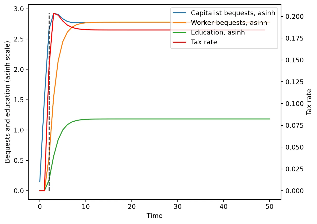
Such an economy shifts from a two-class division based on capital ownership to one in which both groups own capital. The two population groups remain, and they need not hold equal wealth. The critical transition occurs because capitalists eventually find it optimal to impose a tax on themselves to finance public education. As a result, and as wages continue to increase, workers are eventually able to leave bequests and thus also become capital owners. Instead of detailing the exact process (see the reference), we will simulate the economy for a set of parameters.
In the paper, it is assumed that: * \(h_{t+1}(0) = 1,\) * \(h^\prime_{t+1}(0) = \gamma < \infty,\) * \(\lim_{e_t \rightarrow \infty}h^\prime_{t+1}(e_t) = 0.\)↩︎