2 The OLG model
2.1 Introduction
Based on Croix and Michel (2009).
We have studied the Ramsey model, which predicts that the path derived from the competitive equilibrium is optimal. One of the main features of this model is that agents have an infinite horizon: they live forever and optimise considering an infinite horizon.
The overlapping generations model changes this hypothesis and focuses on the life cycle: agents make decisions regarding how much to consume and save for retirement. That is, the OLG model assumes that agents work until some age and then retire.1 A focus of the OLG model is intergenerational redistribution, which allows us to study:
- social security,
- education policies and
- public debt.
The main departure with respect to the Ramsey model is that in OLG, agents are heterogeneous. Individuals live for two periods of time, and then die. In the first period, they are young and work. When old, they retire and live from savings. Hence, at any point in time, two types of agents with different budget constraints exist: young and old.2
As we shall see, in this model the competitive path may not be optimal. Consequently, there may be instances in which the utility of all individuals can be increased. Therefore, the OLG model opens the door to government intervention, to reallocate consumption and savings efficiently. The OLG framework also permits the existence of bubbles and fluctuations.
A basic reference for this model is Diamond (1965)
2.2 Preliminaries
In this model, time is discrete and extends from \(t=0, 1, \ldots, \infty.\) Individuals make decisions at points in time. We shall have initial conditions detailing the state of the economy at \(t=0.\)
2.2.1 Individuals live for two periods
The main difference with respect to the Ramsey model is that in the OLG model, individuals live for two periods. Note: this means that, at every point in time, two generations are alive and overlap.
This is relevant: the economy goes on forever but individuals only operate during some periods. Hence, there will be infinite two-period-lived generations. In particular, at \(t=0\), we have a young generation born at \(t=0\) and an old generation born at \(t=-1\). The old generation dies at the end of \(t=0\); at \(t=1\), the generation born at \(t=0\) is old and a new young generation is born. Hence, we can represent the generations diagrammatically —in brackets I have denoted the year in which each generation was born.
| \(t=0\) | \(t=1\) | \(t=2\) | \(t=3\) | \(t=4\) | \(t=5\) |
|---|---|---|---|---|---|
| Old (t=-1) | Die | ||||
| Young(t=0) | Old (t=0) | Die | |||
| Young(t=1) | Old (t=1) | Die | |||
| Young(t=2) | Old (t=2) | Die | |||
| Young(t=3) | Old (t=3) | Die | |||
| Young(t=4) | Old (t=4) | ||||
| Young(t=5) |
Let \(N_t\) denote the size of the young cohort born at \(t\). To simplify the model, we assume that cohort size grows at the constant rate \(n>-1\). Note: fertility and cohort growth are exogenous.
More complex set-ups include endogenous fertility.
Thus,
\[ N_t=(1+n)N_{t-1}. \]
The size of the young cohort is therefore
\[ N_{t} = N_{0}(1+n)^{t}. \]
Because the old cohort at \(t\) has size \(N_{t-1}\), the total living population is \(N_t+N_{t-1}\), not \(N_t\).
2.3 Assumptions
2.3.1 Firms
We assume that a large number of identical firms populate the economy. Firms produce a single, homogeneous good using labour and capital. The production function \(F(K,L)\) has the following properties:
Assumption OLG 1: The production function satisfies the following properties:
- OLG 1.1 \(F(K, L)\) is continuous and defined on \([0,+\infty)^{2},\)
- OLG 1.2 \(F(K, L)\) has continuous derivatives of every required order on \((0,+\infty)^2,\)
- OLG 1.3 The production function is strictly increasing in both arguments: \(F_{i}(K, L) > 0\),
- OLG 1.4 The production function is concave, and its intensive form is strictly concave: \(f^{\prime\prime}(k)<0\) for \(k>0\).
- OLG 1.5 \(F(K, L)\) is homogeneous of degree one.
Note: We do not assume the Inada conditions globally: the CES examples studied below violate one end each (see the steady-state discussion). A sufficient condition for an interior golden rule is introduced locally in that section.
Note: Constant returns to scale make strict concavity of \(F\) on the whole input space impossible: along any ray, output is linear in scale. Concavity of \(F\) and strict concavity of \(f\) provide the curvature used below.
Firms maximise real profits. Since there are many firms competing, in equilibrium they make exactly zero profits. Moreover, in equilibrium factors are paid their marginal productivity. Since the production function \(F\) is homogeneous of degree one, we can write it in intensive terms:
\[ f(k) \equiv F\left(\frac{K}{L},1\right), \quad k \equiv \frac{K}{L}. \tag{2.1}\]
Because markets are competitive, capital earns the rental rate \(r_t=\partial F(K_t,L_t)/\partial K_t\), or \(f^{\prime}(k_t)\) in intensive terms. After depreciation, the gross return on one unit saved is:
\[ r_t=f^{\prime}(k_t), \qquad R_t=1-\delta+r_t=1-\delta+f^{\prime}(k_t). \tag{2.2}\]
The marginal product of labour is given by \(\partial F(K,L)/\partial L.\) In intensive terms, it is equal to:
\[ w_{t} = f(k) - f^{\prime}(k) k. \tag{2.3}\]
2.3.2 Households
Individuals live for two periods. As before, we assume perfect foresight for individuals. Assumption OLG 2 Individuals have perfect foresight.
When young, they are endowed with one unit of labour that they supply inelastically. Assumption OLG 3 Individuals supply one unit of labour inelastically when young. They receive the current wage rate \(w_t\) and allocate this income between:
- current consumption \(c_{t}\),
- savings \(s_{t}\) that are invested in the firms.
Therefore, the budget constraint of a young individual in period \(t\) is:
\[ w_{t} = c_{t} + s_{t}. \]
Once an individual reaches old age in the next period, the individual consumes the gross return on savings and then dies. Old people do not care about anything happening after death. Old-age consumption, \(d_{t+1}\), is determined by the saving choice made when young.
The budget constraint for this period is:
\[ s_{t}(1 - \delta + r_{t+1}) = d_{t+1}. \]
with \(\delta \in (0,1)\) being the capital depreciation rate.
Hence, an individual faces two budget constraints. However, we can collapse both into a unique intertemporal budget constraint.
2.3.2.1 The intertemporal budget constraint
In the economy, we have consumption as the numeraire. It is more convenient for us to combine the two budget constraints corresponding to young and old ages into one single constraint. Starting from
\[ \begin{cases} w_{t} = c_{t} + s_{t} \\ d_{t+1} = s_{t}(1 - \delta + r_{t+1}) = s_{t} R_{t+1} \end{cases} \tag{2.4}\]
where \(R_{t+1} \equiv 1-\delta+r_{t+1}=1-\delta+f'(k_{t+1})\) represents the gross return on savings from \(t\) to \(t+1\), isolate \(s_t\) in the second equation and plug it into the first one:
\[ w_{t} = c_{t} + \frac{d_{t+1}}{R_{t+1}}. \tag{2.5}\]
The intertemporal budget constraint indicates that the total present value of income (\(w_{t}\), the only source of income) equals the total present value of expenditures. The present value of consumption when old \(d_{t+1}\) is discounted using the gross return \(R_{t+1}.\)
Savings will be a function of wages \(w\) and the gross return \(R\). So will consumption at all periods of time.
2.3.2.2 Utility function
We suppose that the life-cycle utility function is additively separable:
\[ U(c,d) = u( c ) + \beta u(d),\, \beta \in(0,1) \tag{2.6}\]
where \(\beta \in (0,1)\) is the psychological discount factor. We assume that \(u( c )\) has the properties
Assumption OLG 4
- OLG 4.1 \(u^{\prime}( c ) > 0,\)
- OLG 4.2 \(u^{\prime \prime} ( c ) < 0,\)
- OLG 4.3 \(\lim_{c \rightarrow 0} u^{\prime}( c) = +\infty,\)
- OLG 4.4 \(\lim_{c\rightarrow+\infty}u'(c)=0.\)
The assumption \(\lim_{c \rightarrow 0} u^{\prime}( c ) = +\infty\) (OLG 4.3) implies that an individual will always have a positive consumption —as long as he has enough income to finance it. Assumption OLG 4.4 (\(\lim_{c\rightarrow+\infty}u'(c)=0\)) is used in the existence proof below, in the case where savings tend to zero as the gross return goes to infinity.
Another important implication of the choice of the utility formulation is that \(c\) and \(d\) are normal goods: the demand is not decreasing in wealth. It follows from additive separability and concavity.
2.3.3 The behaviour of individuals
At time \(t\), young individuals receive their wages, consume and save while maximising the utility function.
\[ \begin{aligned} & \max u(c_{t}) + \beta u(d_{t+1}) \\ & \mathrm{s.t.} \quad w_{t} = c_{t} + s_{t} \\ & \phantom{s.t.} \quad d_{t+1} = R_{t+1}s_{t} \\ & \phantom{s.t.} \quad c_{t} \geq 0, d_{t+1} \geq 0. \end{aligned} \tag{2.7}\]
We have two possibilities to solve this problem:
2.3.3.1 Substitution
First, we can substitute \(c_{t}\) and \(d_{t+1}\) in the utility function, leading to:
\[ u(w_{t} - s_{t}) + \beta u(R_{t+1}s_{t}). \]
This function is strictly concave with respect to \(s_{t}\) because of our assumptions. The solution is the savings function:
\[ s_{t} = s(w_{t}, R_{t+1}). \]
The solution is interior as a consequence of the assumptions, and it is characterised by the first-order condition:
\[ u^{\prime}(w_{t} - s_{t}) = \beta R_{t+1} u^{\prime}(R_{t+1}s_{t}). \tag{2.8}\]
2.3.3.2 Lagrangian
Instead, we can use the intertemporal budget constraint and build the Lagrangian:
\[ \mathcal{L} = u(c_{t}) + \beta u(d_{t+1}) + \lambda_{t}(w_{t} - c_{t} - \frac{d_{t+1}}{R_{t+1}}). \]
The first order conditions imply that:
\[ u^{\prime}(c_{t}) = \lambda_{t}, \quad \beta u^{\prime}(d_{t+1}) = \frac{\lambda_{t}}{R_{t+1}}. \]
Combining both, we obtain Equation 2.8 again: \[ u^{\prime}(c_{t}) = \beta R_{t+1} u^\prime (d_{t+1}). \]
2.4 Intertemporal elasticity of substitution
The intertemporal elasticity of substitution is defined as:
\[ \epsilon_{d_{t+1}, c_{t}} = \frac{ \partial \left( \frac{d_{t+1}}{c_{t}} \right)}{\partial R_{t+1}} \frac{ R_{t+1}}{\left( \frac{d_{t+1}}{c_{t}} \right)}. \tag{2.9}\]
From the Euler equation we have \(u'(c_t)/u'(d_{t+1})=\beta R_{t+1}\). In general, this condition does not make \(d_{t+1}/c_t\) a function of \(R_{t+1}\) alone: both consumption levels can change with the return and wealth. Consequently, the inverse-RRA formula does not follow from an unrestricted total differentiation that holds \(c_t\) fixed.
For CIES (equivalently, isoelastic or CRRA) period utility, homotheticity makes the consumption ratio depend only on the gross return. Let \(d_{t+1}=x_{t+1}c_t\). Then the intertemporal elasticity of substitution becomes:
\[ \epsilon_{d_{t+1}, c_{t}} = \frac{ \partial x_{t+1}}{\partial R_{t+1}} \frac{ R_{t+1}}{x_{t+1}}. \]
For the CIES specification below, this elasticity is constant and equals the inverse of the constant coefficient of relative risk aversion. This mathematical equivalence is useful even though the deterministic model itself contains no risk.
2.4.1 CIES example
We illustrate the previous concept using a constant intertemporal elasticity of substitution utility function:
\[ u(c)= \begin{cases} \dfrac{c^{1-\frac{1}{\sigma}}-1}{1-\frac{1}{\sigma}}, & \sigma>0,\ \sigma\neq1,\\[4pt] \log c, & \sigma=1. \end{cases} \]
In this case, we have the following Euler condition:
\[ u^{\prime}(c_{t}) = \beta R_{t+1} u^{\prime}(d_{t+1}) \implies \frac{d_{t+1}}{c_{t}} = \left( \beta R_{t+1} \right)^\sigma. \]
Therefore, the intertemporal elasticity of substitution is
\[ \epsilon_{d_{t+1}, c_{t}} = \frac{ \partial \frac{d_{t+1}}{c_{t}} }{\partial R_{t+1}} \frac{R_{t+1}}{\color{red}{\frac{d_{t+1}}{c_{t}}}}= \sigma (\beta R_{t+1})^{\sigma-1}\beta R_{t+1} \color{red}{\frac{1}{(\beta R_{t+1})^{\sigma}}} = \sigma. \]
Meanwhile, the coefficient of relative risk aversion
\[ RRA( c ) = - \frac{u^{\prime \prime}( c )}{u^{\prime}( c )}c = \frac{1}{\sigma} = \epsilon^{-1}_{d_{t+1},c_{t}} \]
is the inverse of the intertemporal elasticity of substitution.
2.5 The savings function
The savings function arises by solving:
\[ s(w, R) = \arg \max \left[ u(w-s) + \beta u(Rs) \right]. \]
Taking the first derivative with respect to \(s\) and solving provides an implicit function: the savings function.
\[ u^\prime(w-s)(-1) + \beta u^\prime(Rs)R = 0. \]
Denote this function \(\phi(s,w,R)\):
\[ \phi(s, w, R ) = -u^\prime(w-s)+ \beta R u^\prime(Rs) = 0. \]
Following from the assumption on the utility function, the savings function is continuous and continuously differentiable.
We are interested in determining whether savings increase or decrease with wealth and the gross return.
2.5.1 The effect of wages
We begin by analysing the effect of wages on savings:
\[ \begin{aligned} \frac{\partial s}{\partial w} &= -\frac{\partial\phi/\partial w}{\partial\phi/\partial s} \\ &= \frac{u^{\prime\prime}(w-s)} {u^{\prime\prime}(w-s)+\beta R^2u^{\prime\prime}(Rs)} \\ &= \frac{1}{1+\beta R^2 \frac{u^{\prime\prime}(Rs)}{u^{\prime\prime}(w-s)}} \in (0,1). \end{aligned} \]
We thus have that the marginal propensity to save out of income is between 0 and 1: \(0 < s^{\prime}_{w} < 1,\) which reflects the fact that consumption goods are normal goods.
2.5.2 The effect of the gross return
Similarly, define the local elasticity \(\sigma(d)\equiv-u'(d)/[d u''(d)]\) and compute \(\frac{\partial s(w,R)}{\partial R}\):
\[ \frac{\partial s}{\partial R} = -\frac{ \beta u^{\prime}(d) + \beta R s u^{\prime \prime}(d)}{u^{\prime \prime}( c )+\beta R^{2} u^{\prime \prime}(d)} =- \frac{\beta u^{\prime}(d)\left[1-\frac{1}{\sigma (d)} \right]}{u^{\prime \prime}(c ) + \beta R^{2} u^{\prime \prime}(d)}. \]
Hence, \[ \frac{\partial s}{\partial R} \gtreqqless 0 \quad \mathrm{if} \quad \sigma (d) \gtreqqless 1. \]
Two effects interact in this derivative:
- Wealth effect: if the gross return rises, we obtain more from the same savings and hence become wealthier. We consume more of all goods —\(c_{t}\) and \(d_{t+1}\) are normal goods.
- Substitution effect: it is more profitable to save and consume \(d_{t+1},\) inducing savings.
When the intertemporal elasticity of substitution is lower than 1, the substitution effect is dominated by the income effect. In that case, a rise in the rate of return has a negative effect on savings. When the intertemporal elasticity of substitution is higher than 1, households are ready to exploit the rise in the remuneration of savings by consuming relatively less today. In this case, raising the rate of return boosts savings. When the intertemporal elasticity of substitution is equal to 1 (log utility), the income effect exactly offsets the substitution effect and the gross return does not affect savings.
2.5.2.1 Example using a CIES function
Under a CIES utility, we have that:
\[ s(w,R) = \frac{1}{1+\beta^{-\sigma}R^{1-\sigma}}w, \]
and \[ s^{\prime}_w =\frac{1}{1+\beta^{-\sigma}R^{1-\sigma}} > 0. \]
However, \(s^{\prime}_{R} = - \frac{w \beta^{-\sigma} R^{-\sigma}}{\left(1+\beta^{-\sigma}R^{1-\sigma}\right)^{2}}(1-\sigma)\gtreqqless 0\) depending on \(\sigma \lesseqqgtr 1.\)
Log-utility:
In the case of logarithmic utility, savings are independent of the gross return \(R\) and are linear in wages. Log-utility is a special case of the CIES function when \(\sigma=1.\) In this case, the wealth and substitution effects cancel each other:
\[ s(w,R) = \frac{\beta}{1+\beta}w. \]
2.5.2.2 Example using a CES function
Note: These homothetic preferences represent the same intratemporal trade-off as an appropriate monotonic transformation, so the solution looks similar to the CIES case.
\[ U(c,d) = \left[ \alpha c^{\frac{\epsilon-1}{\epsilon}} + (1-\alpha)d^{\frac{\epsilon-1}{\epsilon}} \right]^{\frac{\epsilon}{\epsilon-1}}. \]
From here, substituting \(c=w-s\) and \(d=Rs\), and solving for the optimal savings we obtain:
\[ \begin{aligned} & \alpha (w-s)^{-\frac{1}{\epsilon}} = (1-\alpha) R (Rs)^{-\frac{1}{\epsilon}} \\ & s = \frac{\left[ \frac{\alpha}{1-\alpha} \right]^{-\epsilon} w}{R^{1-\epsilon} + \left[\frac{\alpha}{1-\alpha} \right]^{-\epsilon}} = \frac{w}{1+\left[ \frac{\alpha}{1-\alpha} \right]^{\epsilon} R^{1-\epsilon}}. \end{aligned} \]
Therefore,
\[ s^{\prime}_{R} = - \frac{w}{\left(1+\left[ \frac{\alpha}{1-\alpha} \right]^{\epsilon} R^{1-\epsilon}\right)^{2}} \left(\frac{\alpha}{1-\alpha}\right)^{\epsilon}(1-\epsilon)R^{-\epsilon}. \]
Then, when \(\epsilon >1\) savings increase with the interest rate: \(s^{\prime}_{R} > 0.\) In that case, the substitution effect dominates. Alternative interpretation: \(\epsilon\) is the elasticity of intertemporal substitutability, hence if it is large, individuals are willing to substitute present consumption for future consumption. For this isoelastic specification, \(1/\epsilon\) is also the curvature coefficient commonly called relative risk aversion. Here, the economic interpretation concerns willingness to substitute consumption across dates, since the model is deterministic.
Conversely, when \(\epsilon <1\), an increase in the interest rate lowers savings: \(s^{\prime}_{R} < 0.\) In that case, the wealth effect dominates. \(\epsilon<1\) also means that \(c\) and \(d\) are relatively difficult to substitute across dates, so their ratio responds little to changes in the return.
2.6 Temporary equilibrium
Before turning to the intertemporal equilibrium and the analysis of the steady state, we study the temporary equilibrium that takes place every period.
We have not discussed the firms, but they follow the same setup as in Ramsey: use capital and labour in a perfectly competitive environment.
We shall work in intensive form: \(k_{t} \equiv \frac{K_{t}}{N_{t}}.\)
Labour market equilibrium: Only young individuals supply labour. Moreover, they do so inelastically. During period \(t\) there are \(N_{t}\) young agents and, hence, the supply of labour is \(N_{t}\). Equating this to labour demand from firms \(L_{t}\) gives the wage rate: \[ w_{t} = \omega\left(\frac{K_{t}}{N_{t}}\right)=\omega(k_{t}). \]
Capital market: Only old individuals own capital. The capital installed at \(t\) is owned by the old, so asset-market clearing requires \[ K_t=N_{t-1}s_{t-1}. \] Competitive firms pay the rental rate \(r_t=f'(k_t)\). Including the undepreciated principal, old households receive \[ N_{t-1}d_t=N_{t-1}R_ts_{t-1}=R_tK_t, \qquad R_t=1-\delta+f'(k_t). \]
Good market: Finding the equilibrium for this market departs from the otherwise similar Ramsey case. Remember that we have two types of agents: young and old. Total production is given by:
\[ Y_{t} = F(K_{t}, N_{t}) = \color{red}{N_{t}} f(k_{t}). \]
Available goods combine current output and undepreciated capital. They are used for the consumption of the old and young and for next period’s capital. Thus, the resource constraint is
\[ Y_t+(1-\delta)K_t=N_{t-1}d_t+N_tc_t+K_{t+1}. \] Equivalently, if gross investment is \(I_t\equiv K_{t+1}-(1-\delta)K_t\), then \[ Y_t=N_{t-1}d_t+N_tc_t+I_t. \]
Asset-market clearing for the savings of the young requires \(K_{t+1}=N_ts_t\), so equivalently \[ Y_t+(1-\delta)K_t=N_{t-1}d_t+N_t(c_t+s_t). \]
We can verify this identity from factor payments: \[ \begin{aligned} N_t(c_t+s_t) &= N_tw_t \\ &= N_t\left[f(k_t)-k_tf^\prime(k_t)\right] \\ &= Y_t-K_tf^\prime(k_t). \end{aligned} \]
\[ N_{t-1}d_t=R_tK_t=\left[1-\delta+f'(k_t)\right]K_t. \] Net investment is \(\Delta K_t\equiv K_{t+1}-K_t=I_t-\delta K_t\). Savings finance ownership of the entire next-period capital stock, \(K_{t+1}=N_ts_t\), not just net investment.
A temporary equilibrium is a set \(\\{w_{t}, R_{t}, K_{t}, L_{t}, Y_{t}, k_{t}, I_{t}, c_{t}, s_{t}, d_{t}\\}\) that satisfies:
\[ \begin{aligned} w_{t} = \omega(k_{t}), \\ R_t = 1-\delta+f'(k_t), \\ L_{t} = N_{t}, \\ Y_{t} = N_{t}f(k_{t}), \\ Y_t+(1-\delta)K_t=N_{t-1}d_t+N_tc_t+K_{t+1}, \\ K_t=N_{t-1}s_{t-1}, \qquad K_{t+1}=N_ts_t, \\ I_t=K_{t+1}-(1-\delta)K_t, \\ c_{t} = w_{t} - s_{t}, \\ s_{t} = s(\omega(k_{t}),R_{t+1}), \\ d_t=R_ts_{t-1}. \end{aligned} \]
The existence of a temporary equilibrium is guaranteed because the functions are single-valued.
2.7 Intertemporal equilibrium with perfect foresight
The equilibrium equation that links two consecutive periods is the capital accumulation equation. In particular, the savings of young individuals at period \(t\) are transformed into productive capital at \(t+1.\)
Note: in this model, it is useful to write the equations first in aggregate terms and then convert them to its intensive-form representation.
\[ K_{t+1} = N_{t}s_{t} = N_{t} s\left( \omega(k_{t}), R_{t+1} \right). \]
In intensive form:
\[ k_{t+1} = \frac{K_{t+1}}{\color{red}{N_{t+1}}} = \frac{N_{t}}{\color{red}{N_{t+1}}} s\left( \omega(k_{t}), R_{t+1} \right) = \frac{1}{1+n}s\left( \omega(k_{t}), R_{t+1} \right). \]
Finally, we can incorporate capital-market equilibrium and perfect foresight by replacing \(R_{t+1}\) with \(1-\delta+f^{\prime}(k_{t+1})\):
\[ k_{t+1} =\frac{1}{1+n}s \left( \omega(k_{t}), 1-\delta+f^{\prime}(k_{t+1}) \right). \]
Intertemporal equilibrium (under perfect foresight): Given an initial capital stock per young worker \(k_0=K_0/N_0\), an intertemporal equilibrium is a sequence of temporary equilibria that satisfies for all \(t\geq0\) the equation:
\[ k_{t+1} =\frac{1}{1+n}s \left( \omega(k_{t}), 1-\delta+f^{\prime}(k_{t+1}) \right). \]
Note: Croix and Michel (2009, 20–27) discusses the existence and uniqueness of the intertemporal equilibrium.
2.7.1 Existence of an intertemporal equilibrium
The existence of at least one next-period equilibrium is guaranteed by the properties of the functions. The proof is involved and is presented below. Having an intertemporal equilibrium means having a solution for \(k_{t+1}\) in the equation
\[ k_{t+1} = \frac{1}{1+n}s(\omega(k_t), 1-\delta+f^\prime (k_{t+1})), \]
where \(k_t\) is predetermined at \(t.\)
NoteProof
For \(w>0\), the proof uses the following inequality for savings: \[ 0<s\left(w,1-\delta+f'(k)\right)<w. \]
In words, individuals have positive savings but save only part of their total income. If \(w=0\), then \(s=0\) and \(k=0\) is the solution.
Next, define \[ H(k,w)=(1+n)k-s\left(w,1-\delta+f'(k)\right)=0. \]
Basically, here we are using the definition of an intertemporal equilibrium. Having an intertemporal equilibrium is then equivalent to finding a \(k\) satisfying the previous equation.
We use the intermediate value theorem to show that at least one solution exists. First, we analyse the behaviour of \(H(k,w)\) when \(k\) tends to \(+\infty.\)
From \(0<s\left(w,1-\delta+f'(k)\right)<w\), we have
\[ 0 < \frac{s(w,1-\delta+f'(k))}{k} < \frac{w}{k}. \]
Limit when \(k \rightarrow +\infty\)
Keeping \(w\) fixed, the limit of \(\frac{w}{k}\) when \(k \rightarrow +\infty\) is 0. Then,
\[ \lim_{k \rightarrow +\infty} \frac{s(w,1-\delta+f'(k))}{k} = 0. \]
Consequently,
\[ \begin{aligned} \lim_{k \rightarrow +\infty}\frac{H(k,w)}{k} &= \lim_{k \rightarrow +\infty} \left[(1+n)-\frac{s(w,1-\delta+f'(k))}{k}\right] \\ &= 1+n > 0. \end{aligned} \]
Limit when \(k \rightarrow 0\)
When \(k\) tends to zero, we distinguish two cases regarding \(f'(k)\) and therefore the gross return. It can be that either
- Case \(\lim_{k\rightarrow0}f'(k)=f'(0)>0\) and finite. Then, the function \(s(w,1-\delta+f'(k))\) is well defined and positive and we have:
\[ \begin{aligned} \lim_{k \rightarrow 0}H(k,w) &= \lim_{k \rightarrow 0}\left[(1+n)k-s(w,1-\delta+f'(k))\right] \\ &= -s(w,1-\delta+f'(0)) < 0. \end{aligned} \]
Case \(\lim_{k \rightarrow 0} f^\prime (k) = +\infty.\) Two things can occur in that case.
Savings are positive: \(\lim_{k\rightarrow0}s(w,1-\delta+f'(k))>0\). This case is analogous to the previous one:
\[ \begin{aligned} \lim_{k \rightarrow 0}H(k,w) &= \lim_{k \rightarrow 0}\left[(1+n)k-s(w,1-\delta+f'(k))\right] \\ &<0. \end{aligned} \]
Savings tend to zero: \(\lim_{k\rightarrow0}s(w,1-\delta+f'(k))=0\). In this case, as the gross return goes to infinity, individuals may save an amount tending to zero. This implies that consumption in the second period, \(d\), tends to infinity. To see this, first notice that \(d = [1-\delta+f'(k)]s(w,1-\delta+f'(k)).\) Moreover, from the first order conditions we know that: \[ u'(d)=\frac{u'(w-s)}{\beta[1-\delta+f'(k)]}. \]
and hence \[ \lim_{k\rightarrow0}u'(d)=\lim_{k\rightarrow0}\frac{u'(w-s)}{\beta[1-\delta+f'(k)]}=0. \]
Hence, \(u^\prime (d)\) tends to zero which means that \(d\) goes to infinity. Therefore:
\[ \lim_{k\rightarrow0}[1-\delta+f'(k)]s(w,1-\delta+f'(k))=+\infty. \]
We also know that \(0 < f^\prime (k) k < f(k)\) because \(f^\prime (k) k + \omega(k) = f(k)\) and \(\omega(k) > 0.\) Therefore, for a bounded \(0<k<1\) we also have \(f^\prime (k) k < f(1).\) Hence, for \(k<1\):
\[ \begin{aligned} \frac{s(w,1-\delta+f'(k))}{k} &= \frac{f'(k)s(w,1-\delta+f'(k))}{f'(k)k} \\ &> \frac{f'(k)s(w,1-\delta+f'(k))}{f(1)}. \end{aligned} \]
Then,
\[ \lim_{k\rightarrow0}\frac{s(w,1-\delta+f'(k))}{k}=+\infty \]
and \[ \frac{H(k,w)}{k}=1+n-\frac{s(w,1-\delta+f'(k))}{k}<0 \]
for small \(k\).
2.7.2 Uniqueness of the intertemporal equilibrium
Having established that at least one level \(k_{t+1}\) exists that solves the equation, we would like it to be unique, thus having a unique equilibrium. Otherwise, for some level \(k\) there would be multiple values for \(k_{t+1}\) (meaning multiple values for the savings). Individuals lack a coordinating mechanism to select any of these equilibria.
We show that the intertemporal elasticity of substitution \(\sigma\) is important in determining uniqueness. In particular, with CIES utility, \(\sigma\geq1\) is sufficient for uniqueness. We will revisit this issue later.
We have used the intermediate value theorem to show that solutions exist. Moreover, the proof shows that \(H(k,w)<0\) for sufficiently small positive \(k\) and \(H(k,w)>0\) for sufficiently large \(k\). Therefore, if \(H(k,w)\) is strictly increasing in \(k\), there is exactly one solution to \(H(k,w)=0\). Hence, we would have a unique solution. This means that, given \(k_t\), we can find a unique value \(k_{t+1}\).
If we take the derivative of \(H(k,w)\) with respect to \(k\), we obtain:
\[ 1+n - s^{\prime}_R f^{\prime \prime}(k). \]
Consequently, for \(H\) to be strictly increasing it is sufficient to impose:
Assumption OLG 5: \[ 1+n - s^{\prime}_R f^{\prime \prime}(k) > 0. \]
And then, \(k_{t+1} = g(k_{t}).\)
In particular, this condition indicates that the effect of the gross return on savings should not be too negative.
Moreover, if OLG 5 is satisfied, then \(k_{t+1}\) is increasing in \(k_t\). Indeed,
\[ k_{t+1}=\frac{1}{1+n}s(\omega(k_t),R(k_{t+1})). \]
and
\[ \frac{\mathrm{d}k_{t+1}}{\mathrm{d}k_t} =\frac{\overbrace{s'_w\omega'(k_t)}^{>0}} {1+n-s'_R\underbrace{R'(k_{t+1})}_{=f''(k_{t+1})<0}}>0, \]
and \(k_{t+1}\) increases in \(k_{t}.\)
Important
Hence, if the function \(H\) is strictly increasing, the solution is unique. This condition depends on the sign of:
\[ \frac{\partial H(k_{t+1},w_t)}{\partial k_{t+1}} =1+n-s'_R f''(k_{t+1}). \]
Finally, we can use a more restrictive —but easier to work with— assumption that ensures a unique solution for the intertemporal equilibrium. Assumption OLG 5 states:
\[ 1+n - s^{\prime}_R f^{\prime \prime}(k) > 0. \]
Therefore, it is sufficient to have
\[ s^{\prime}_R \geq 0 \]
meaning that savings increase with the gross return. This behaviour is readily verified when the intertemporal elasticity of substitution is at least one. Then, for CIES utility, \(\sigma\geq1\) is sufficient for monotonic dynamics and a unique next-period equilibrium.
We have different cases:
- \(s^\prime_{R} = 0\), which happens under log-utility. In this case, \(s^\prime_{R} = 0 > \frac{1+n}{R^\prime(k_{t+1})}\) and \(H(k_{t+1})\) is always increasing.
- \(s^\prime_{R} >0\), the intertemporal elasticity of substitution is greater than 1 and individuals are willing to trade off higher future consumption against present consumption. Savings increase to consume more in the future. Then, clearly \(s^\prime_{R} > 0 > \frac{1+n}{R^\prime(k_{t+1})}.\)
- If \(s'_R<0\), uniqueness can still hold, but it requires the negative return effect on saving not to be too strong.
2.7.3 Possible multiple equilibria and non-monotonic dynamics
When \(s'_R<0\), the sufficient condition for uniqueness may fail; it does not follow that multiplicity must occur. For some utility and production parameters, the implicit equilibrium relation can bend backward and admit several values of \(k_{t+1}\) for the same \(k_t\). This section is based on Groth (2016, 92–93).
Such values are alternative, self-fulfilling perfect-foresight equilibria. If all agents coordinate on one anticipated \(k_{t+1}\), its associated return determines saving and asset-market clearing realizes that same capital stock. A low CIES parameter \(\sigma<1\) makes this possibility more likely because saving decreases with the return, but it is neither necessary nor sufficient by itself.
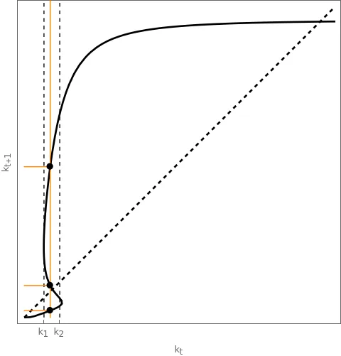
The figure illustrates the shape that can generate this multiplicity. Multiplicity means that perfect foresight does not select a unique equilibrium; it does not mean that realized outcomes differ from expectations within a selected equilibrium.
2.8 Steady states
We assume that the intertemporal equilibrium exists and is unique. As noted when characterising uniqueness, for CIES utility, \(\sigma\geq1\) is a sufficient condition. Therefore, the dynamics of capital are given by:
\[ k_{t+1}=\frac{1}{1+n}s(\omega(k_t),1-\delta+f'(k_{t+1})). \]
Hence, \(k_{t+1}\) is an implicit function of \(k_{t}\):
\[ k_{t+1} = g(k_{t}). \]
The steady states of this economy can be found solving the previous equation for \(k_{t+1} = k_{t}=\bar{k}.\)
\[ \bar{k}=\frac{1}{1+n}s\left(\omega(\bar{k}),1-\delta+f'(\bar{k})\right). \]
2.8.1 Steady state with \(\bar{k}=0\)
A steady state with \(\bar{k}=0\) is only possible if \(f(0)=0\) or, equivalently, \(\omega(0)=0.\) We may call this steady state an autarky steady state. In that case, since \(\omega(0)=0\) and we know that individuals save a fraction of their income:
\[ s(\omega(0),R(0))=s(0,R(0))=0. \]
Hence, given zero capital, savings equal zero and capital remains there, constituting a steady state.
Alternatively, if it is possible to produce without capital (CES production function with large enough substitutability), the autarkic steady state does not exist.
2.8.1.1 Example of the autarkic steady state
Take \(F(K,L)=(\alpha K^{\rho} + (1-\alpha)L^{\rho})^{\frac{1}{\rho}}\) and \(u( c ) = \log( c ).\) Furthermore, assume a low elasticity of substitution, \(\rho << 0.\) In intensive form, production equals:
\[ f(k_{t}) = (\alpha k_{t}^{\rho} + (1-\alpha))^{\frac{1}{\rho}}. \]
Wages and savings are:
\[ \begin{aligned} \omega(k_{t}) &= (1-\alpha)(\alpha k^\rho + (1-\alpha))^{\frac{1}{\rho}-1} \\ s_{t} &= \frac{\beta}{1+\beta}w_{t}. \end{aligned} \]
Then, capital accumulation becomes:
\[ k_{t+1} = \frac{1}{1+n}\frac{\beta}{1+\beta}(1-\alpha)\left[\alpha k_{t}^\rho + 1 - \alpha \right]^\frac{1-\rho}{\rho}. \]
With low substitutability, \(\rho < 0\), zero is always a possible steady state. There can be two additional, positive steady states depending on the curvature of \(k_{t+1}.\)
Similarly, the Cobb-Douglas case \(\rho \rightarrow 0\) also has zero as a steady state. However, it is unstable.
2.8.2 Other steady state
The economy can also present interior steady states with \(\bar{k}>0.\) Unlike the Ramsey model, here we can have stable and unstable steady states, as we shall see. Moreover, the configuration varies depending on the production and utility functions.
Two steady states, autarky and positive This is a common configuration that arises, for instance, under a Cobb-Douglas production function and log-utility. Other functions can also exhibit this behaviour, particularly those with similar functional forms.
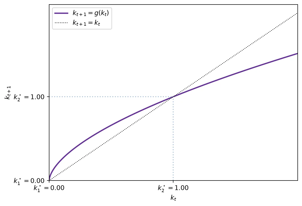
Single, non-autarky steady state This steady state is characterised by a unique positive capital level \(\bar{k}>0\). This configuration requires \(f(0) > 0\). With a CES production function, capital and labour must be sufficiently substitutable, that is, \(0<\rho<1\): \((\alpha k^\rho+(1-\alpha))^{1/\rho}\).
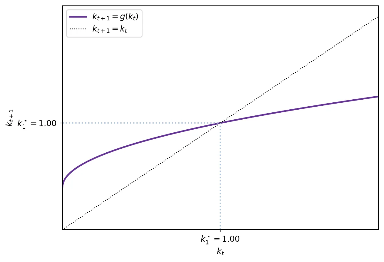
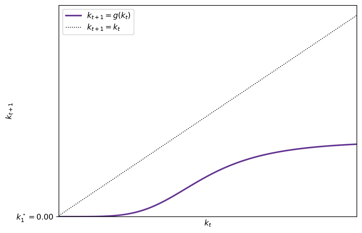
Only an autarky steady state In this case, \(f(0) = 0\) is required so that the autarky steady state can exist. Moreover, it requires \(g(k)<k\) for every \(k>0\). This type of setup can arise with \(\rho<0\), that is, when capital and labour are gross complements and the transition curve is sufficiently low.
2.9 Stability of the steady state
This model can feature one or several steady states. This depends on the characteristics of the production and utility functions.
Under the sufficient condition used above, \(g\) is increasing, so a trajectory cannot cross a fixed point and is monotonic over time. We impose the following condition (Croix and Michel 2009, 25):
\[ \forall c>0, \quad u^\prime( c ) + c u^{\prime \prime}( c ) \geq 0 \Leftrightarrow \sigma( c ) \geq 1. \]
Because the dynamics are monotonic, capital can converge either to \(0, \bar{k}\in (0,+\infty),\) or \(+\infty.\)
2.9.1 The economy never goes to \(k = +\infty\)
This is equivalent to saying that, starting with a high level of capital \(k_0\), the dynamics imply \(k_{t+1}<k_t\).
First, we have that:
\[ g(k)=\frac{1}{1+n}s\left(\omega(k),1-\delta+f'(\underbrace{g(k)}_{k_{t+1}})\right)<\frac{\omega(k)}{1+n}. \]
This holds because savings \(s\) are always a fraction of wages \(\omega.\)
Second, we show that:
\[ \lim_{k \rightarrow +\infty}\frac{g(k)}{k} = 0. \]
To see the intuition for this limit, assume for a moment it holds. Then, it must be that for large enough \(k,\, g(k) = k_{t+1} < k_{t}\) and the dynamics are decreasing and converge to some \(\bar{k}.\) In this case, \(\bar{k}\) is the largest steady state, and because the dynamics are monotonic, the economy never goes to the other side of the steady state.
We show next that \(\lim_{k \rightarrow +\infty}\frac{g(k)}{k} = 0.\) We do so by showing that \(\lim_{k \rightarrow +\infty} \color{green}{\frac{\omega(k)}{k}} = 0.\)
NoteProof
We start by noting that:
\[ \color{green}{\frac{\omega(k)}{k}} = \color{red}{\frac{f(k)}{k}} - \color{blue}{f^\prime (k)} \leftarrow \omega(k) = f(k) - f^\prime (k) k. \]
When \(k\rightarrow+\infty\), the first term \(\color{red}{f(k)/k}\) admits a finite nonnegative limit, which we call \(\mathcal{l}_1\). This is because:
- \(\color{red}{\frac{f(k)}{k}} > 0.\)
- \(\color{red}{\frac{f(k)}{k}}\) is decreasing: \[ \begin{aligned} \frac{\partial [f(k)/k]}{\partial k} &= \frac{f^\prime(k)k-f(k)}{k^2} \\ &= -\frac{f(k)-f^\prime(k)k}{k^2} \\ &= -\frac{\omega(k)}{k^2}<0. \end{aligned} \]
The second term \(\color{blue}{f^\prime (k)}\) is decreasing and positive, thus it admits a limit \(\mathcal{l}_{2}\) when \(k \rightarrow +\infty.\)
Apply the mean value theorem evaluated at \(k\) and \(2k\):
\[ f(2k) - f(k) = (2k-k)f^\prime(k(1+\theta)), \quad \mathrm{with}\, \theta \in (0,1). \]
Then,
\[ \frac{2f(2k)}{2k} - \frac{f(k)}{k} = f^\prime(k(1+\theta)) \]
Taking the limit when \(k \rightarrow +\infty\) we obtain \(2\mathcal{l}_{1}-\mathcal{l}_{1} = \mathcal{l}_{2} \implies \mathcal{l}_{1} = \mathcal{l}_{2}.\)
Finally,
\[ \lim_{k \rightarrow + \infty}\color{green}{\frac{\omega(k)}{k}} =\lim_{k \rightarrow +\infty}\color{red}{\frac{f(k)}{k}} - \color{blue}{f^\prime (k)}= \mathcal{l}_{1} - \mathcal{l}_{2} = 0. \]
Since \(\lim_{k \rightarrow +\infty} \color{green}{\frac{\omega(k)}{k}}=0\) and \(\frac{g(k)}{k} < \color{green}{\frac{\omega(k)}{k}}\) then \(\lim_{k \rightarrow +\infty}\frac{g(k)}{k} = 0.\) In conclusion, if the initial value of capital is large enough, the dynamics are decreasing and converge to a finite nonnegative steady state. The limit can be zero when zero is the only steady state.
2.10 Examples
2.10.1 Example 1: Log-utility and Cobb-Douglas
Suppose that \(u(c,d) = \log ( c ) + \beta \log(d)\) and \(f(k_t) = Ak_t^\alpha.\)
The wage rate is given by \[ w_t=f(k_t)-k_tf'(k_t)=(1-\alpha)Ak_t^\alpha \]
and the savings function is obtained solving \[ u^\prime(w_{t} - s_{t}) = \beta R_{t+1} u^\prime (R_{t+1}s_{t}). \]
Rearranging and isolating \(s\) we are left with the savings function
\[ s_{t} = \frac{\beta}{1+\beta}w_{t}. \]
The dynamics are given by the capital accumulation law
\[ k_{t+1} = \frac{1}{1+n}s_{t} = \frac{1}{1+n}\frac{\beta}{1+\beta}w_{t} = \frac{1}{1+n}\frac{\beta}{1+\beta}(1-\alpha)Ak_{t}^\alpha. \]
The model with log-utility and Cobb-Douglas production functions has two steady states: zero and a unique positive steady state. We can solve for them:
\[ \begin{aligned} \phi &\equiv \frac{\beta(1-\alpha)A}{(1+n)(1+\beta)}, \\ \bar{k} &= \phi\bar{k}^\alpha \\ \implies \bar{k} &\in \left\{0,\ \phi^\frac{1}{1-\alpha}\right\}. \end{aligned} \]
The dynamics are depicted in Figure 2.2.
Local dynamics: stability
We check the stability of the two steady states using the first derivative evaluated at the steady state. Note: in general we would use the Jacobian matrix, but the OLG model has only one equation in one variable.
Remember that a fixed point of a one-dimensional discrete-time system is locally asymptotically stable if \(|g'(\bar{k})|<1\) and unstable if \(|g'(\bar{k})|>1\). It is hyperbolic when \(|g'(\bar{k})|\neq1\); the equality case requires further analysis.
In our case:
\[ g(k) = k_{t+1} = \frac{1}{1+n}\frac{\beta}{1+\beta}(1-\alpha)Ak_{t}^\alpha \] \[ g^\prime(k) = \frac{1}{1+n}\frac{\beta}{1+\beta}(1-\alpha)\alpha Ak_{t}^{\alpha-1}> 0. \]
Then
\[ \bar{k}=0 \implies g^\prime (0) = + \infty \quad \rightarrow \mathrm{unstable} \] \[ \bar{k}=\phi^\frac{1}{1-\alpha} \implies g^\prime(\phi^\frac{1}{1-\alpha}) = \phi \alpha \phi^\frac{\alpha-1}{1-\alpha} = \alpha \in (0,1) \quad \rightarrow \mathrm{stable}. \]
Only an autarky steady state In this case, \(f(0) = 0\) is required so that the autarky steady state can exist. Moreover, it requires \(g(k)<k\) for every \(k>0\). This type of setup can arise with \(\rho<0\), that is, when capital and labour are gross complements and the transition curve is sufficiently low.
2.10.2 Log-utility and CES technology
Under a CES specification, \(y_t=A[\alpha k_t^\rho+(1-\alpha)]^{1/\rho}\), with \(\rho<1\) and \(\rho\neq0\), wages are given by \[ \omega_t=A(1-\alpha)\left[\alpha k_t^\rho+1-\alpha\right]^{\frac{1-\rho}{\rho}}. \]
Hence, the dynamics of capital are governed by:
\[ \begin{aligned} k_{t+1} = g(k_t) &= \frac{1}{1+n}s_t \\ &= \frac{\beta A(1-\alpha)}{(1+n)(1+\beta)} \left[\alpha k_t^\rho+1-\alpha\right]^\frac{1-\rho}{\rho}. \end{aligned} \]
The curve \(g(k)\) is increasing:
\[ g'(k)=\frac{\beta A(1-\alpha)}{(1+n)(1+\beta)}\alpha(1-\rho) \left[\alpha k^\rho+1-\alpha\right]^{\frac{1-2\rho}{\rho}}k^{\rho-1}>0. \]
Depending on the value of \(\rho\) we can have different configurations regarding the steady states. Ultimately, what matters is the concavity of the function \(g(k_{t}).\)
\[ \begin{aligned} g^{\prime\prime}(k_t) &= -\frac{\beta A(1-\alpha)(1-\rho)\alpha}{(1+n)(1+\beta)} \\ &\quad \times \left[\alpha k^\rho+1-\alpha\right]^\frac{1-3\rho}{\rho} k^{\rho-2} \\ &\quad \times \left[\rho\alpha k^\rho+(1-\alpha)(1-\rho)\right]. \end{aligned} \]
2.10.2.1 Unique steady state, \(\bar{k} > 0\)
If \(\rho \in (0,1)\), the second derivative is clearly negative, and \(g\) is concave. Moreover, \(g(0)>0\), so \(\bar{k} = 0\) cannot be a steady state:
\[ \begin{aligned} g(k_t) &= \frac{\beta A(1-\alpha)}{(1+n)(1+\beta)} (\alpha k^\rho+1-\alpha)^\frac{1-\rho}{\rho}, \\ \implies g(0) &= \frac{\beta A(1-\alpha)^{1/\rho}} {(1+n)(1+\beta)} > 0. \end{aligned} \]
In that case, the economy displays a unique steady state, and it is globally stable.
See Figure 2.3.
2.10.2.2 Unique \(\bar{k}=0\) or multiple steady states
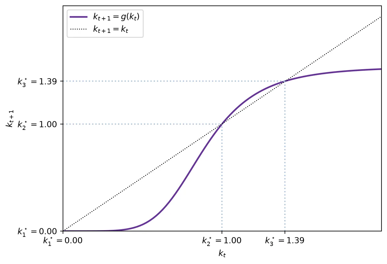
If \(\rho < 0,\) the function \(g(k)\) changes concavity. In particular, there exists a level \(\hat{k}\) such that: \[ g^{\prime \prime}(k) > 0\, \mathrm{if} \, k < \hat{k}. \] \[ g^{\prime \prime}(k) < 0\, \mathrm{if} \, k > \hat{k}. \] with \[ \hat{k} = \left( - \frac{(1-\alpha)(1-\rho)}{\rho \alpha}\right)^\frac{1}{\rho} > 0 \, \mathrm{since}\, \rho <0. \] Moreover, \(g(0)=0\) so \(\bar{k}=0\) can be a steady state.
In this case, there are two sub-cases:
If \(g(k)<k\) for every \(k>0\), equivalently \(\frac{\omega(k)}{k}<(1+n)\frac{1+\beta}{\beta}\) for every \(k>0\), then the transition curve is always below the 45-degree line. Then, there is one unique steady state: \(\bar{k}=0.\) The economy converges towards this unique steady state. We can derive the condition above from: \[\begin{aligned} k_{t+1} < k_{t} & \implies \frac{1}{1+n}s\left(\omega(k_{t}),R_{t+1}\right) < k_{t} \implies \\ \frac{1}{1+n}\frac{\beta}{1+\beta}w_t < k_{t} & \implies \frac{w_{t}}{k_{t}} < (1+n)\frac{1+\beta}{\beta}. \end{aligned} \]
If \(g(k)>k\) for some \(k>0\), equivalently \(\frac{\omega(k)}{k}>(1+n)\frac{1+\beta}{\beta}\) there, then the S-shaped transition curve crosses the 45-degree line twice at positive capital levels \(\bar{k}_a<\bar{k}_b\), in addition to the zero steady state.
- All trajectories starting at \(k_0 < \bar{k}_{a}\) converge to \(\bar{k}=0\) and \(\bar{k}=0\) is locally stable in the range \([0,\bar{k}_{a}].\) The steady state with \(\bar{k}=0\) is a poverty trap: whenever the economy starts with a low enough level of capital, it will always converge towards the \(\bar{k}=0\) steady state.
- Trajectories starting at \(k_0=\bar{k}_{a}\) remain at \(\bar{k}_{a}\). This steady state is unstable.
- Finally, trajectories starting with \(k_0 > \bar{k}_{a}\) converge towards \(\bar{k}_{b}\), which is a locally stable steady state in \((\bar{k}_{a}, +\infty).\)
See Figure 2.4 and Figure 2.1.
2.11 Solved example
Suppose that production can be parametrized using the following Cobb-Douglas specification:
\[ Y = F\left(K_t, L_t\right) = K_t^\frac{1}{2}L_t^\frac{1}{2}. \]
Furthermore, assume full depreciation, \(\delta=1\), and the following period utility function:
\[ u(c_t) = \frac{c_t^{1-\frac{1}{3}}-1}{1-\frac{1}{3}} \]
where the intertemporal elasticity of substitution is \(3\).
We can compute the production function, wage, and capital rental rate in intensive form as:
\[ \begin{aligned} f(k_t) &= k_t^{1/2} \\ w_t &= \frac{1}{2}k_t^{1/2} \\ r_t &= \frac{1}{2}k_t^{-1/2} \end{aligned} \]
Similarly, the savings function can be derived from the Euler equation as follows:
\[ \begin{aligned} u^\prime(w_t - s_t) &= \beta R_{t+1} u^\prime(s_t R_{t+1}) \implies \\ \implies (w_t -s_t)^\frac{-1}{3} &= \beta R_{t+1} (R_{t+1} s_t)^\frac{-1}{3} \implies \\ \implies (w_t - s_t) &= \beta^{-3} R_{t+1}^{-2} s_t \implies \\ s_t &= \frac{w_t}{1+\beta^{-3}R_{t+1}^{-2}} \end{aligned} \]
Therefore, the capital accumulation equation is:
\[ \begin{aligned} k_{t+1} &= \frac{1}{1+n} \frac{w_t}{1+\beta^{-3}R_{t+1}^{-2}}, \\ w_t &= \frac{1}{2}k_t^{1/2}, \qquad R_{t+1}=\frac{1}{2}k_{t+1}^{-1/2}, \\ \implies k_{t+1} &= \frac{1}{1+n} \frac{\frac{1}{2}k_t^{1/2}}{1+4\beta^{-3}k_{t+1}}, \\ \frac{1}{2}k_t^{1/2} &= (1+n)k_{t+1}\left(1+4\beta^{-3}k_{t+1}\right), \\ k_{t+1} &= \frac{-(1+n) +\sqrt{(1+n)^2+8(1+n)\beta^{-3}k_t^{1/2}}} {8(1+n)\beta^{-3}}. \end{aligned} \]
We can then show that the autarky steady state exists. Indeed, because we have \(f(0) = 0\), then \(\bar{k} = 0\) is a steady state. The economy has a second steady state. It is most conveniently characterised by a third-degree polynomial. Nevertheless, let’s sketch the process, knowing that a steady state solves \(k_t = k_{t+1} = \bar{k}.\) To simplify the notation, in what follows I will write \(k\) instead of \(\bar{k}.\)
\[ \begin{aligned} 4\beta^{-3}k^2+k-\frac{k^{1/2}}{2(1+n)}&=0. \end{aligned} \]
Letting \(x=k^{1/2}\geq0\) gives \[ x\left(4\beta^{-3}x^3+x-\frac{1}{2(1+n)}\right)=0. \] Thus, \(k=0\) is a steady state. The expression in parentheses is strictly increasing in \(x\), is negative at zero, and tends to infinity. It therefore has exactly one positive root, which gives exactly one positive steady state.
The derivative of the dynamic function with respect to \(k_t\) is:
\[ \frac{\partial k_{t+1}}{\partial k_t} = \frac{1}{4\sqrt{k_t}\sqrt{(1+n)\left(1+n+\frac{8\sqrt{k_t}}{\beta^{3}}\right)}} \]
At \(k_t=k_{t+1}=0\), the right derivative is \(+\infty\), so the zero steady state is unstable. The derivative need not be below one at every positive \(k_t\), but at the positive fixed point the steady-state equation implies \[ g'(\bar{k})=\frac{4\beta^{-3}\bar{k}+1}{2(8\beta^{-3}\bar{k}+1)}\in\left(\frac14,\frac12\right). \] The unique positive steady state is therefore locally stable. In fact, the plot corresponds to Figure 2.2.
2.12 The golden-rule level of capital
The first welfare theorem states that a competitive equilibrium is Pareto optimal. However, the first welfare theorem has two requisites the Diamond model does not meet: a finite number of goods and a finite number of agents. Therefore, the allocation resulting from the competitive equilibrium may not be Pareto optimal. This section is based on Croix and Michel (2009, Ch. 2) and Groth (2016).
In the Diamond model —and different from the Ramsey model—, the capital stock on the balanced growth path may exceed the golden-rule level. This implies that a permanent increase in consumption is possible.
When discussing the golden-rule level of capital, we are not interested in how consumption is divided between the old and the young. Rather, we seek to maximise aggregate consumption that can be sustained period after period. This criterion determines the efficient capital stock, but not how consumption should be allocated between the young and old; that distribution requires a separate welfare criterion. First, let \(\mathfrak{C}_t\) represent total consumption:
\[ \mathfrak{C}_t \equiv C_t + D_t. \] The economy-wide resource constraint dictates that total production is either consumed or invested:
\[ \mathfrak{C}_t + K_{t+1} = F(K_t, N_t)+ (1-\delta)K_t. \]
Alternatively, aggregate consumption per unit of labour is:
\[ \begin{aligned} \mathfrak{c}_t \equiv \frac{\mathfrak{C}_t}{N_t} &= \frac{F(K_t, N_t) +(1-\delta)K_t - K_{t+1}}{N_t} = \\ & = f(k_t) + (1-\delta)k_t - (1+n)k_{t+1}. \end{aligned} \]
The golden-rule level of the capital-labour ratio \(k^{\mathcal{GR}}\) is the value of the capital-labour ratio \(k\) that results in the highest possible sustainable level of consumption per unit of labour. The fact that it is sustainable requires that it is replicable forever. For this reason, we consider the steady state with \(k_{t+1} = k_t = \bar{k}\). The resource constraint at the steady state simplifies to:
\[ \bar{\mathfrak{c}} = f(\bar{k})-(\delta + n)\bar{k} \equiv \mathfrak{c}(k). \]
We maximise this function with respect to \(\bar{k}\):
\[ \mathfrak{c}^\prime(\bar{k}) = f^\prime (\bar{k}) - (n+\delta) = 0 \]
The fact that \(\mathfrak{c}^{\prime \prime}(\bar{k}) = f^{\prime \prime}(\bar{k})<0\) assures that we have the maximum.
Assuming that \(n+\delta >0\) and that \(f\) satisfies:
\[ \lim_{k \rightarrow +\infty} f^\prime(k) < n+ \delta < \lim_{k \rightarrow 0} f^\prime(k), \tag{2.10}\]
then \(\mathfrak{c}^\prime(\bar{k}) = f^\prime (\bar{k}) - (n+\delta) = 0\) has a solution in \(\bar{k}\) and it is unique.
Remark (Inada conditions: sufficient, not necessary). The textbook Inada conditions on the production function,
\[\begin{align*} \lim_{K \rightarrow 0} F^\prime_{K}(K, L) &= \lim_{L \rightarrow 0} F^\prime_{L}(K, L) = +\infty \\ \lim_{K \rightarrow +\infty} F^\prime_{K}(K, L) &= \lim_{L \rightarrow +\infty} F^\prime_{L}(K, L) = 0, \end{align*}\]
imply Equation 2.10 whenever \(n+\delta>0\), so they are sufficient for a unique interior golden rule. They are not necessary, and they are not assumed elsewhere in this chapter: Cobb–Douglas satisfies both ends, while the CES examples above violate one end each (finite \(f'(0)\) when \(\rho<0\); \(f(0)>0\) with \(f'\to\alpha^{1/\rho}>0\) at infinity when \(0<\rho<1\)). Hence, the golden-rule level of capital is given by:
\[ f^\prime(k^{\mathcal{GR}}) = n + \delta. \]
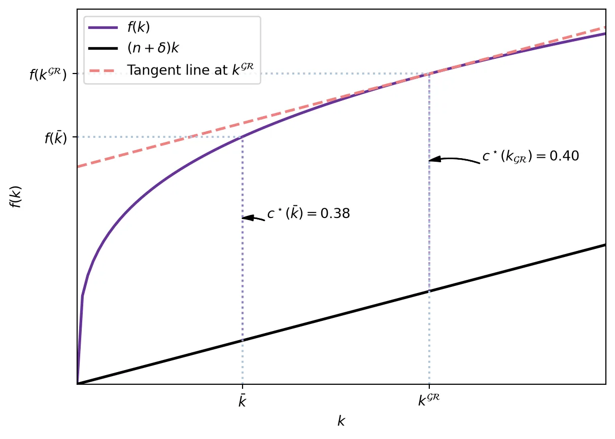
The highest sustainable consumption level per unit of labour is obtained when, at steady state, the net marginal productivity of capital equals the growth rate of the economy.
2.12.1 Over- and under-accumulation of capital
The golden-rule level of capital is given by \(f^\prime(k) = n+\delta.\) However, in the decentralised economy, the steady-state level of savings is highly unlikely to coincide with it. For instance, with log utility and \(f(k)=Ak^\alpha\), the decentralized positive steady state satisfies \[ f'(\bar{k})=\frac{\alpha(1+n)(1+\beta)}{\beta(1-\alpha)}, \] which generally differs from \(n+\delta\).
If the steady-state level of the economy is such that \(f^\prime (\bar{k}) < n+ \delta,\) the economy has accumulated too much capital: if \(f^\prime (\bar{k}) < f^\prime(k^{\mathcal{GR}}) \implies \bar{k} > k^{\mathcal{GR}}.\) Conversely, if the marginal product at the competitive steady state satisfies \(f'(\bar{k})>n+\delta\), then the economy lacks capital relative to the golden rule.
2.12.1.1 Improving the situation: dynamic inefficiency
Suppose that the decentralised economy reaches a situation of overaccumulation of capital, that is, \(f'(\bar{k})<n+\delta\). It is possible to improve upon it by means of redistribution. Simply, a planner could order young individuals to save less, as to reach \(k^{\mathcal{GR}}.\) Doing so increases the resources available for consumption per worker, which can be allocated between the old and young to support a Pareto improvement. In subsequent periods, the economy would remain at \(k^{\mathcal{GR}}\), which maximises sustainable aggregate consumption per worker.
In particular, assume we impose a lump-sum tax on all young individuals and we transfer it to the old generation. The transfer is fully consumed (old individuals gain utility from consuming it). Suppose the transfer is one good from each young to the old. There are \(1+n\) young individuals per old individual, so the old receive \(1+n\) goods. Let’s repeat this scheme every period.
- The young transfer one good to the old
- Consumption of the young does not change because they refrain from saving.
- In the future, they receive \(1+n\), which is the gross return on their implicit PAYG contribution.
- In the competitive market, they would have obtained the gross return \(R=1-\delta+f'(k)\).
- Under overaccumulation, \(f'(k)<n+\delta\) is equivalent to \(R<1+n\), so the PAYG gross return is larger.
At the same time, old individuals are also better off. In the first period, when the reform is introduced, they consume more. Later generations obtain a higher return for the tax they pay, leaving them better off, too.
When organising such scheme is possible, we say that the competitive economy was dynamically inefficient.
Note: it is possible to solve the dynamic inefficiency introducing money. Young individuals would exchange goods for paper notes with the expectation of exchanging them back again when old.
2.12.1.2 Dynamic efficiency
In the opposite case, when \(\bar{k} < k^\mathrm{GR}\), reaching the golden-rule level of capital requires increasing it. Suppose we are at time \(t_0\). Increasing the capital to \(k^{\mathcal{GR}}\) would certainly improve consumption for all generations \(t > t_0\). However, young individuals at \(t_0\) should forgo some consumption to save more and build the necessary capital. Hence, the consumption of the young generation at \(t_0\) necessarily decreases. Our policy of improving utility for all individuals fails in this case.
We call such situations dynamically efficient: it is impossible to increase the utility of all generations.
2.12.2 Example
We use a log-utility and Cobb-Douglas case to illustrate over- and under-accumulation of capital.
\[ U(c,d) = \log( c ) + \beta \log (d) \] \[ f(k)= Ak^\alpha. \]
The golden-rule level of capital dictates that total consumption per worker should be maximised. Using the resource constraint:
\[ \max \mathfrak{c}_t=f(k_t)+(1-\delta)k_t-(1+n)k_{t+1}. \]
Evaluating it at the steady state yields:
\[ \max \mathfrak{c} = f(k) - (n+\delta)k \implies f^\prime(k^{\mathcal{GR}}) = n+\delta. \]
Hence, in our case:
\[ A \alpha {k^{\mathcal{GR}}}^{\alpha-1} = n + \delta \implies k^{\mathcal{GR}} = \left(\frac{A\alpha}{n+\delta}\right)^\frac{1}{1-\alpha}. \]
In the decentralised economy, we have that:
\[ k_{t+1}=\frac{1}{1+n}s\left(\omega(k_t),1-\delta+f'(k_{t+1})\right) =\frac{1}{1+n}\frac{\beta}{1+\beta}A(1-\alpha)k_t^\alpha. \]
Hence, the steady-state level of capital is:
\[ \bar{k}=\frac{A\beta(1-\alpha)}{(1+n)(1+\beta)}\bar{k}^\alpha \implies \bar{k}=\left[\frac{A\beta(1-\alpha)}{(1+n)(1+\beta)}\right]^{\frac{1}{1-\alpha}}. \]
We have capital over-accumulation if: \(\bar{k} > k^{\mathcal{GR}} \implies \frac{(n+\delta) \beta}{(1+n)(1+\beta)} > \frac{\alpha}{1-\alpha}.\)
Check Romer (2018, 89–90) for an empirical discussion about the dynamic efficiency.
2.13 The Central Planner
Suppose now, instead, that a central planner is in charge of organising consumption and investment for all individuals. The planner operates by aggregating individual utility, discounting future generations at the rate \(\gamma.\) Note: \(\gamma\) is the discount rate of future generations, not how young people discount old-age utility.
Her utility considers the utility of all generations, including the initial old generation, which owns the initial aggregate capital stock \(K_0\) (equivalently, each initial old agent owns \((1+n)k_0\)).
2.13.1 Planner’s utility
Planner’s utility reads:
\[ \sum_{t=-1}^\infty \gamma^t U(c_t, d_{t+1}). \]
Note that, although the planner can decide any allocation, she must respect the resource constraint:
\[ f(k_t) + (1-\delta) k_t = c_t + \frac{1}{1+n} d_t + (1+n)k_{t+1}. \]
Assume that \(U(c_t, d_{t+1})\) is separable: \(U(c_t, d_{t+1}) = u(c_t) + \beta u(d_{t+1}).\) Expanding the utility of the planner, we can reformulate it in more convenient terms:
\[ \begin{aligned} \sum_{t=-1}^\infty \gamma^t\left[u(c_t)+\beta u(d_{t+1})\right] &= \gamma^{-1}u(c_{-1})+\gamma^{-1}\beta u(d_0) \\ &\quad +u(c_0)+\beta u(d_1) \\ &\quad +\gamma u(c_1)+\gamma\beta u(d_2)+\ldots \\ &= \sum_{t=0}^\infty \gamma^t \left[u(c_t)+\frac{\beta}{\gamma}u(d_t)\right] \\ &\quad +\gamma^{-1}u(c_{-1}). \end{aligned} \]
The term \(\gamma^{-1}u(c_{-1})\) represents the consumption of the generation born at \(t=-1\), but since it is a constant it will not affect the maximisation.
Hence, the planner’s problem is now how to allocate consumption between the young and old that are alive during period \(t\).
2.13.2 Maximisation
We use a substitution to obtain the planner’s optimal allocation, namely, the Euler equation;
\[ \begin{aligned} &\max_{k_{t+1},c_t,d_t}\ \sum_{t=0}^\infty\gamma^t \left[u(c_t)+\frac{\beta}{\gamma}u(d_t)\right] \\ &\mathrm{s.t.}\quad f(k_t)+(1-\delta)k_t =c_t+\frac{d_t}{1+n}+(1+n)k_{t+1}. \end{aligned} \]
\[ \begin{aligned} \max_{c_t,k_{t+1}}\quad &\sum_{t=0}^\infty \gamma^t \left[u(c_t)+\frac{\beta}{\gamma}u(d_t)\right] \\ \text{s.t.}\quad d_t &= (1+n)\left[f(k_t)+(1-\delta)k_t -(1+n)k_{t+1}-c_t\right]. \end{aligned} \]
Taking derivatives and equating them to zero yields:
\[ \gamma^t u^\prime(c_t) = \gamma^t \frac{\beta}{\gamma} u^\prime(d_t)(1+n) \] \[ \begin{aligned} \gamma^t\frac{\beta}{\gamma}u^\prime(d_t)(1+n)^2 &= \gamma^{t+1}\frac{\beta}{\gamma}(1+n) \\ &\quad \times u^\prime(d_{t+1}) \left[f^\prime(k_{t+1})+1-\delta\right]. \end{aligned} \]
Combining both equations we get the Euler equation:
\[ u^\prime (c_t) = \beta u^\prime (d_{t+1})\left(f^\prime (k_{t+1}) + 1 -\delta \right). \]
The planner’s Euler equation coincides with the decentralised one, where \(R_{t+1}=1-\delta+f'(k_{t+1})\).
However, the planner also allocates consumption between the young and the old at time \(t\). \[ \gamma^t u^\prime(c_t) = \gamma^t \frac{\beta}{\gamma} u^\prime(d_t)(1+n) \]
In the centralised equilibrium, the planner also trades off the consumption of different cohorts alive at time \(t\). This condition has no decentralized counterpart because finitely lived individuals value only their own life-cycle consumption; an old individual does not value the contemporaneous young cohort’s consumption.
2.13.3 Steady state and modified golden rule
Using the fact that \[ \begin{aligned} \gamma^t\frac{\beta}{\gamma}u^\prime(d_t)(1+n)^2 &= \gamma^{t+1}\frac{\beta}{\gamma}(1+n) \\ &\quad \times u^\prime(d_{t+1}) \left[f^\prime(k_{t+1})+1-\delta\right] \end{aligned} \]
we can easily characterise the steady state knowing that \(d_t = d_{t+1} = \bar{d}, k_t = k_{t+1} = \bar{k}.\)
\[ f'(\bar{k})=\frac{1+n}{\gamma}-1+\delta. \]
This equation provides us with the modified golden rule: the level of capital that maximises the planner’s utility. Clearly, if \(\gamma=1\), the planner attributes the same weight to all generations and we recover the golden rule: \(f^\prime(k) = n + \delta.\) As we discussed before, it is quite unlikely the decentralised equilibrium converges towards the golden rule (modified or not).